Linear Predictions: Substitute, Interpret, and Check the Range

A scatterplot may suggest a straight-line relationship, but a numerical prediction requires an equation. Regression uses an explanatory value that you know to predict a response that you do not yet know. Keep that direction straight: predicting y from x is different from solving backward for an x that would produce a desired y.

From Linear Form to a Prediction

If the relationship between x and y appears linear, a linear regression model can approximate it. The model is a linear equation using the explanatory variable x to predict the response variable y. Write the predicted response as y-hat, $\hat{y}$, because it is a prediction rather than an observed response:

Here a is the y-intercept, b is the slope of the regression line, and x is the explanatory value supplied to the model. Identify the variables and units before substitution. Observations can differ from their predictions even when a line is a useful summary of the relationship.

Worked Example: Delivery Time

A delivery service records route distance x in kilometers and delivery time y in minutes. Its generated observations are:

Distance (km)	1	2	4	6	8	10
Time (min)	11	12	19	22	29	32

The pattern is approximately straight and upward. Suppose the service uses the stated model $\hat{y}=8+2.5x$. This is a supplied model, not a claim that this equation is the least-squares fit to the displayed observations. Its intercept is 8 minutes, slope is 2.5 minutes per kilometer, and explanatory value is route distance.

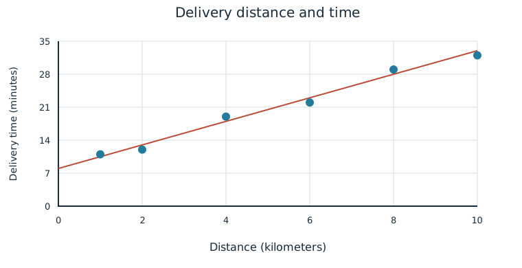
For a 4-kilometer route, substitute x=4:

The model predicts an 18-minute delivery. The displayed 4-kilometer observation is 19 minutes, so its observed time differs from the prediction. Do not replace y-hat by the observed value or reverse the equation to report a distance when a time was requested. A prediction is a model result for a specified explanatory value.

Interpolation and Extrapolation

Interpolation predicts a response for an explanatory value within the interval of x-values used to determine the regression line. Extrapolation uses an explanatory value beyond that interval. The observed response range does not decide which kind of prediction you are making; compare the proposed x with the observed x interval.

For the stated delivery model, an 8-kilometer prediction is interpolation because 8 is within 1–10 kilometers. It gives $\hat{y}=8+2.5(8)=28$ minutes. A 20-kilometer prediction gives 58 minutes but is extrapolation because 20 lies beyond the observed distance interval. The arithmetic still works; the evidence for extending the relationship is weaker. A 50-kilometer extrapolation is still farther beyond the data and generally less reliable than a nearby extrapolation.

Extrapolation can fail because the process changes. Long routes may use highways, require additional stops, or enter a different service area. Those mechanisms are not learned by observing only short routes. Interpolation also carries uncertainty; a fitted line does not guarantee an individual’s observed response.

Check Form, Range, and Context

Before reporting a prediction, inspect whether the observed form is approximately linear, identify explanatory and response variables, substitute the requested explanatory value, and state the predicted response with units. Then classify the prediction by the observed x-range and explain any material limitation.

If the data bend strongly, a convenient line can give systematically inappropriate predictions even for x-values inside the observed interval. For example, the complete pairs (1,1),(2,4),(3,9),(4,16) trace a curve. Interpolation only locates the input within the observed interval; it does not fix a poorly chosen model form. A useful prediction report combines arithmetic with the relationship’s shape and scope.

Independent Practice

Use the information in each question to make your own calculation, representation, or argument. Explain what your result means in its setting.

Original generated practice for the Fall 2026 course.

Read the model before using it

A rental shop uses $\hat y=12+3x$, where x is route distance in kilometers and y is rental duration in minutes. The observed distance interval is 1–9 kilometers.

Part a

Identify the explanatory variable, response variable, predicted response notation, a, and b. Explain the direction of prediction.

Your reasoning

Worked answer and rubric

Predict an observed-range rental

Use $\hat y=12+3x$, with x in kilometers and predicted y in minutes. Observed x-values range from 1 to 9 kilometers.

Part a

Calculate and interpret the predicted duration for x=6 kilometers. Show substitution and classify the prediction as interpolation or extrapolation.

Your reasoning

Worked answer and rubric

Arithmetic beyond the data

Use $\hat y=12+3x$, based on x-values from 1 to 9 kilometers.

Part a

Predict rental durations at 10 and 30 kilometers. Classify both predictions and explain which extends farther beyond the evidence.

Your reasoning

Worked answer and rubric

A within-range input on a curve

A proposed line is intended for the full pairs (1,1),(2,4),(3,9),(4,16).

Part a

Does x=2.5 being inside the observed interval establish that a linear regression model is appropriate? Explain using the shape and the meaning of interpolation.

Your reasoning

Worked answer and rubric

Route predictions with a stated model

A rental shop records the generated pairs (route kilometers, rental minutes)=(1,14),(2,15),(3,19),(4,21),(5,25). The shop proposes the supplied model $\hat y=10+3x$; it is not presented as a recovered historical or least-squares equation.

Part a

Explain whether the scatterplot’s form reasonably supports using a linear model as an approximation. Identify x, y, y-hat, a, and b.

Your reasoning

Part b

Calculate and interpret the predicted rental duration for a 4.5-kilometer route. Classify the prediction and explain how its predicted value differs conceptually from an individual observed value.

Your reasoning

Part c

Calculate predictions at 6 and 20 kilometers. Classify each and compare their reliability using the observed interval.

Your reasoning

Worked answer and rubric