FFR: Probability Problems Solved with Taylor Series
This original textbook reading covers part of the AP topic. Follow the AP course outline for complete topic instruction and practice.
Section 2
FFR: Probability Problems Solved with Taylor Series
For a standard normal distribution probability problem, the Taylor Series can be used to solve for the probability of an event occurring.
Before jumping into the Calculus, we need to first look at how probability is defined for a normal distribution problem.
Standard Normal Distribution Function
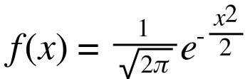
This is the function for a standard normal distribution, and the graph of this function is on the following page.
Important things to know about a standard normal distribution graph is
- the total area under the curve is equal to 1
- the probability of obtaining a value greater than a is equal to the area under the curve on the interval [a, ∞). image 2
- the probability of obtaining a value less than a is equal to the area under the curve on the interval (-∞, a]. image 3
- the probability of obtaining a value between a and b is equal to the area under the curve on the interval [a, b]. image 4
Graph 7-3-1
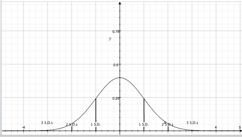
The typical ‘Bell Curve’ of the standard normal distribution function. As stated before, the area underneath the curve is equal to 1.
The vertical lines drawn inside the curve show how many standard deviations away that value is from the average, or mean value.
Read all original image captions
Image 1
The typical ‘Bell Curve’ of the standard normal distribution function. As stated before, the area underneath the curve is equal to 1.
The vertical lines drawn inside the curve show how many standard deviations away that value is from the average, or mean value.
Image 2
Graphical representation of the probability of obtaining a value greater than a.
Image 3
Graphical representation of the probability of obtaining a value less than a.
Image 4
Graphical representation of the probability of obtaining a value between a and b.
Since the value of probability is equal to the area under the curve on some interval, the probability value can be written as the integral of the standard normal distribution function.
Probability Formula
P(a<x<b) = 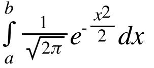
where a and b are the standards of deviation of the event of probability.
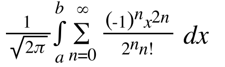
And since it is an exponential function, the integral can be further modified to be written as an integral of a Taylor series for the exponential function, or
P(a<x<b) = 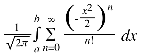 , simplified as
= 
Example 7.3.1
Scoring between 120 and 130 is defined as being between 2 and 3 standards of deviation away from the mean value, or
a = 2, b = 3
Plugging those values into the formula, we then evaluate
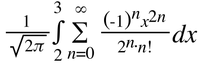
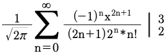

Solving the expression, the probability is about 2%.
Gallery 1.1 Bell Curve for Example 7.3.1
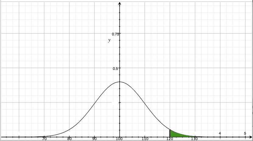
This graph shows the distribution of IQ based on the data provided in example 7.3.1.
Read all original image captions
Image 1
This graph shows the distribution of IQ based on the data provided in example 7.3.1.
Glossary and deeper reading · 5 refreshers
These editorial refreshers supplement the reading. Definitions and examples are added guidance; original source wording and recorded answers remain in their original context.
-
Taylor series
A Taylor series is the infinite power series built from a function’s derivatives at a chosen center. Its coefficients are the derivatives at the center divided by the corresponding factorials. For example, eˣ has Taylor series 1+x+x²/2!+x³/3!+⋯ centered at 0. A Taylor series represents the function only where convergence and the vanishing remainder justify that equality.
-
Normal distribution in integration
A normal distribution is a continuous bell-shaped probability model determined by a mean and a positive standard deviation. The standard normal model has mean 0 and standard deviation 1. For example, the probability that a standard normal variable lies between 0 and 1 is the integral of its density over that interval. The full density has total area 1, and interval areas rather than single-point heights give probabilities.
-
Function
A mathematical function assigns exactly one output to each input in its domain. Inputs can share an output, but one input cannot have two different outputs. For example, f(x)=x² assigns the output 9 to both 3 and −3. Function notation names the rule and its input; f(3) means the output when the input is 3.
-
Interval
An interval is a set of real numbers containing every number between any two of its members. Parentheses exclude an endpoint, while square brackets include it. For example, (1,4] includes 4 and every number between 1 and 4, but excludes 1. An infinite endpoint always uses a parenthesis because infinity is not a real endpoint.
-
Integral
Integration can mean accumulating a function over an interval or finding an antiderivative. A definite integral gives a number, while an indefinite integral represents a family of antiderivatives. For example, integrating 2x indefinitely gives x²+C, and integrating it from 0 to 2 gives 4. The Fundamental Theorem of Calculus connects these two operations under its hypotheses.