Seperable Differential Equations
This original textbook reading covers part of the AP topic. Follow the AP course outline for complete topic instruction and practice.
Section Overview
Section 3
Separable differential equations are some of the most basic differential equations one can encounter. Regardless of this designation they are also extremely common.
Separable differential equations take the form
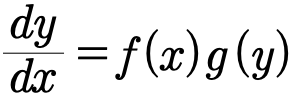
To solve them one uses a technique called separation of variables. In the technique one groups the differentials with their corresponding variables. Doing this to the equation gives us
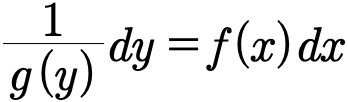
To solve this all that’s necessary is to now integrate both sides and isolate y.
Let’s look at a couple examples to see what this technique looks like.
Example 8.3.1
Solve the following differential equation using separation of variables.
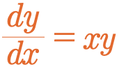
The first thing to do here is determine what type of DE we have. Since we can rearrange our equation to give us
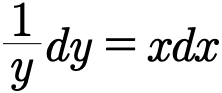
If we integrate the above equation we get that
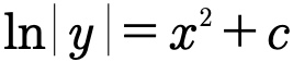
Which after solving for y gives our final solution
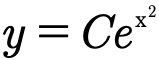
In the above examples two things happened which you may not be familiar with. The first is the absolute value in the natural logarithm. This arises because if y were to be negative the logarithm would fail to work. To fix this issue an absolute value is added.
The second thing is the coefficient on the bottom. The coefficient is made by absorbing the constant of integration formed after integrating.
Example 8.3.1
Determine if the following differential equation is separable. If the equation is separable solve it using separation of variables.
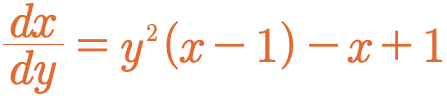
To begin this problem we have to determine that the given differential equation is separable. To do this we just need show that the equation can be written in the form
If we pull out a negative one from the equation we get

After grouping terms we then have
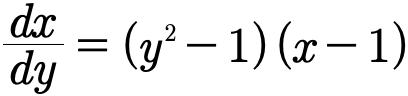
which can then be expressed in the form of a separable equation
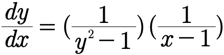
Now that we have a separable equation we can use separation of variables to solve for the dependent variable y.
Since we’re using separation of variables we must group together the proper functions with their corresponding differentials.

Integrating both sides gives the equation

Here y can not be solved for using regular means of symbol manipulation. Since this is the case we will just leave it be.
Solutions in which our dependent variable can not be explicitly defined are not uncommon when doing differential equations and one should not fret if they find one. To solve these computers are often used since it can be extremely troublesome to do them by hand.
Occasionally when solving using separation of variables it is possible to lose a solution. This usually occurs as a result of division by zero at some point while finding a solution to the differential equation in question. The next example will demonstrate a situation in which this happens.
Example 8.3.3
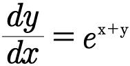
Use separation of variables to find the general solution to the given differential equation. Determine which solutions, if any, were excluded during the process.
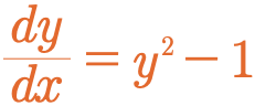
The first order of business is to solve this differential equation. To do this we simply apply the techniques we’ve been studying in this section.
Since the equation is already in the form a separable equation we can just go ahead and group
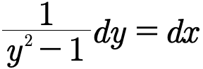
The left hand side can be broken up using partial fraction decomposition
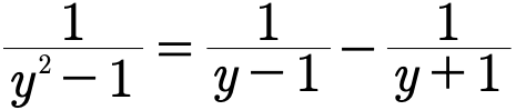
so
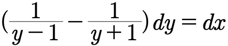
After integrating the equation then becomes

Using logarithm rules the left side can be combined to give
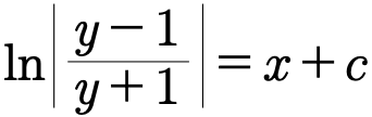
Using the rules of absolute values and raising both sides by to e we get that
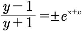
From here we can let
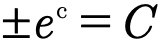
And finally solve for y
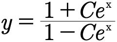
To figure out if this definition of y excludes any solutions we must now look at the original differential equation.
If you let
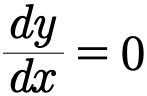
Then

Which implies that
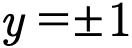
Now if we let
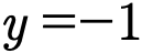
in the solution to our differential equation we get that
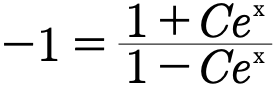
which rearranged is

Implying that
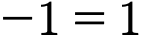
Because the above statement is not true, letting y=-1 is not part of our solution we found but since we know it is a solution to the differential equation we solved the solution used above must have fallen out while we applied separation of variables.
In the above example we lost a solution to our differential equation in the process of looking for its general solution. If you noticed there is a single step in which we divided by y+1. Since letting y=-1 in that case causes division by zero it forced us to exclude -1 as a solution in our final answer.
Review 1.3 Separable Differential Equations
Question 1 of 5 · 0 correct
Determine if the following is a separable differential equation.
Supplementary Image to Example 8.3.3
Read all original figure notes
This Graph
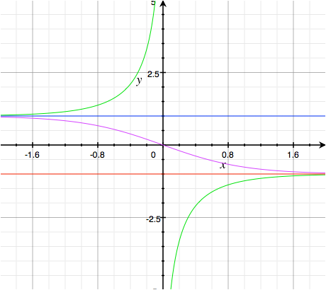
This graph has plotted on it several different curves which satisfy the general solution to the differential equation in example 8.3.3. Each curve here satisfies a different IVP (Initial Value Problem), a topic discussed later.
Limits
Solutions to curves on this graph behave in different ways at the limits. These different behaviors will be classified later on in the book.
y=-1
The solution formed by the line y=-1 is marked in red. Like y=1, y=-1 forms somewhat of a boundary between different solutions. This will be a common feature in graphs of DE solutions.
Glossary and deeper reading · 3 refreshers
These editorial refreshers supplement the reading. Definitions and examples are added guidance; original source wording and recorded answers remain in their original context.
-
Separation of variables
Separation of variables solves certain differential equations by placing the dependent and independent variables on opposite sides. For y′=g(x)h(y), rewrite dy/h(y)=g(x) dx where h(y)≠0 and integrate. For example, y′=xy leads to ln|y|=x²/2+C for nonzero solutions. Check any solutions lost by division, such as y=0 in this example.
-
Differential equation
A differential equation relates an unknown function to one or more of its derivatives. A solution is a function that makes the equation true throughout an appropriate interval. For example, y′=2x has solutions y=x²+C. An initial condition can select a particular member of a family of solutions.
-
Differential
For a differentiable function y=f(x), the differential dy is defined as f′(x) dx. It represents the tangent-line estimate of the output change associated with an input change dx. For example, y=x² at x=3 and dx=0.01 gives dy=6·0.01=0.06. The actual change in y can differ from this linear estimate.