Partial Differentiation
Beyond this AP Calculus course
This original textbook reading covers part of the AP topic. Follow the AP course outline for complete topic instruction and practice.
This reading includes verified answer corrections and explicitly stated clarifications.
Section 4
Partial Differentiation
What happens when you need to take the derivatives of a surface? The derivative as we have come to understand it tells us the instantaneous change of a curve but a surface at any point has more than a single dimension is it moving along. Since the derivative is defined only in terms of a single variable we then can’t use it for a surface. The partial derivative is the solution to this problem.
To take the partial derivative of some function we let all but the variable we wish to take the derivative of be constant. In this way the partial derivatives becomes a measure of the instantaneous rate of change in only a particular direction.
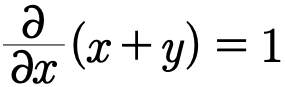
Notationally this operation is commonly indicated by

or

Which tells us to hold all variables besides x constant and differentiate by x.
Gallery 1.2 Looking at partial derivatives
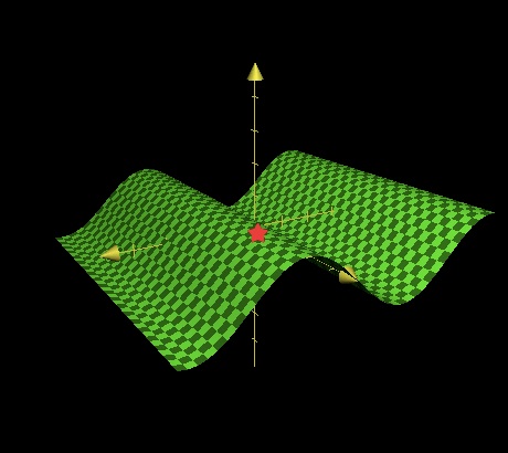
At the point marked with a star the partial with respect to y and the partial with respect to x can be shown to be separate by looking at appropriate cross sections.
Read all original image captions
Image 1
At the point marked with a star the partial with respect to y and the partial with respect to x can be shown to be separate by looking at appropriate cross sections.
Image 2
In the zx-plane a very distinct sine wave exists. Taking the partial of this function with respect to x would give you a cosine since sine defines the cross section.
Image 3
In the zy-plane we would only have lines. Holding x constant while taking the partial of the function which defines the surface in the first image would result in a zero which is indicative of the fact that zy cross sections are lines.
Example 8.4.1
Compute the partial derivative with respect x of the given function.
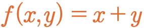
Here we are taking the partial derivative of f with respect to x. This means that we take the derivative of the function with respect to x and treat everything else as constant.
Writing this out then we have

Since y is a constant under the partial
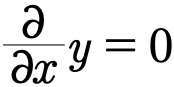
and since x is what we’re taking the partial with respect to it is treated as a variable which means that
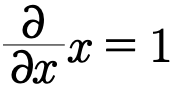
Putting this together gives us that
Example 8.4.2
Compute the partial derivative with respect to y of the following function

This problem is pretty much like the previous. Here though instead of taking the partial with respect to x we will be taking the partial with respect to y.
Since we are taking the partial with respect to y we will be pretending that everything besides y is constant and treating y as we would in a normal variable. Applying the partial derivative we than have that

Since only y is being treated as a variable
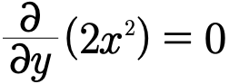
Since the other terms contain y we will have to treat them normally keeping in mind that z is constant since we’re taking the partial derivative of the function with respect to y.

Putting everything together we have that
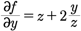
Of course we won’t always be dealing with taking only a single partial derivative of a function. Often times we will be taking multiple partial of the same function after one another. A common notation used to represent this is

or
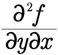
Which tells us that we will be taking a partial with respect to x and then the partial with respect to y of some function f one after another.
Example 8.4.3
Compute

for the function
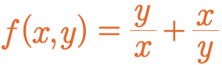
This problem is similar to the rest except now we have to apply two partials sequentially. Using the notation

We work from left to right starting with the partial with respect to x then take the partial with respect to y.
Starting with the partial with respect to x then we have that

The next thing that needs to be done is to take the partial with respect to y

And that’s it!

Chapter 6 Problems
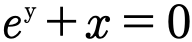
- Implicitly derive the following functions.


- Determine if the given differential equation is linear and state its order.

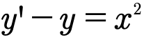
Clarified version of part (c): the displayed differential expression is set equal to zero. This supplies a complete equation for classification.
- Determine if the given function is a solution to the given differential equations.




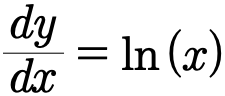
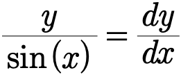
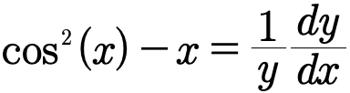
- Use separation of variables to solve the following differential equations.
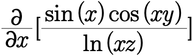
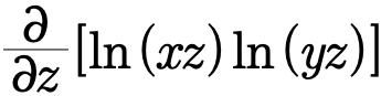
- Compute the given partial derivatives.


Glossary and deeper reading · 3 refreshers
These editorial refreshers supplement the reading. Definitions and examples are added guidance; original source wording and recorded answers remain in their original context.
-
Derivative
A derivative gives the instantaneous rate of change of a function with respect to its input. At a point, it is the finite limit of the difference quotient when that limit exists. For example, the derivative of x² is 2x, so the tangent slope at x=3 is 6. A derivative function collects those rates across the inputs where the function is differentiable.
-
Function
A mathematical function assigns exactly one output to each input in its domain. Inputs can share an output, but one input cannot have two different outputs. For example, f(x)=x² assigns the output 9 to both 3 and −3. Function notation names the rule and its input; f(3) means the output when the input is 3.
-
Instantaneous rate of change
An instantaneous rate of change is the limiting average rate around one input when that limit exists. For a differentiable function, it is its derivative at that input. For example, position s(t)=t² meters has instantaneous rate 4 meters per second at t=2 seconds. The rate’s units are output units per input unit.