Fourier Series fvvffFfasfForF
Beyond this AP Calculus course
This original textbook reading covers part of the AP topic. Follow the AP course outline for complete topic instruction and practice.
This reading includes verified answer corrections and explicitly stated clarifications.
Section Overview
- The Definition of a Fourier Series
- Square Wave Example
- Graphing Fourier Series
Section 4
Fourier Series fvvffFfasfForF
An important type of series which you may encounter later on is called a Fourier Series a type of series which are intimately related to a subject called Fourier Analysis. Fourier Series are used to model functions which have periodic behavior and as a result they often find use in the physical sciences.
A Fourier Series is a specific type of Trigonometric Series defined by the expression

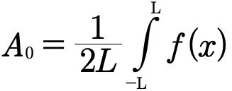
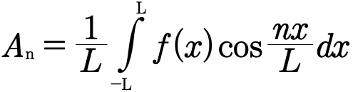
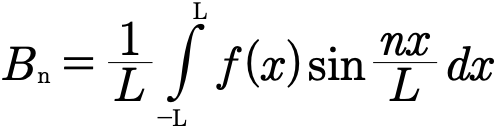
In a Fourier Series the coefficients and the outside term become something very specific. They become defined as follows
 a
Here  is some function which is periodic over some interval which can be integrated and
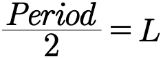
 is defined through the period of our function
 so that

or more clearly
Now that we have the definitions we have a very powerful tool. Using these definitions can be a little confusing though so will now be do an example.
Example 3.4.1
Using the defined function and the given period compute the Fourier Series for that function.

To begin with let’s take a quick look at the function we are asked to create a Fourier Series for.
The first part of the functions definition just gives us it’s value for certain values of x. The function  is equal to one when x is between zero and two and equal to zero when x is between 2 and 4.
The second part of the definition tells us that this function is periodic. In particular this function repeats itself every time 4 units has passed by. This is important because it gives us the value of it’s L.
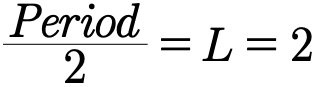
If you recall the definition of a Fourier Series you will remember we need to now solve for two coefficients and a constant. We will start with the constant, it’s usually the easiest to solve for.
If you recall it is defined by the equation
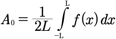
Since we know what L is we get
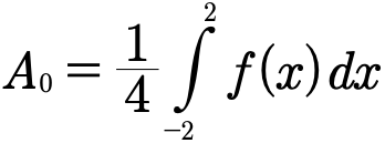
Now things get a little tricky. You may have noticed that our function  has two different values over the interval we’re integrating over. To solve this all we have to do is split up the integral.
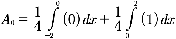
Since the integral of zero is equal to zero all we’re left with is the integral of one which is easily done.
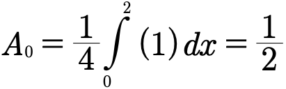
Now that we have our constant we can move onto our coefficients. We will first determine the value of  then determine the value of
 .
For  we will first recall the definition
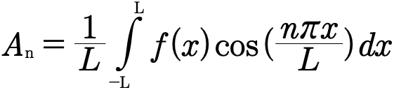
Since we already known what L is we can just plug it in.
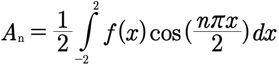
Again we have to deal with our odd function. We will just do the same thing as we did with our constant, split the integral into two.

Since as before we have an integral with zero it will drop and and we’re left only with a single integration to do. Remembering the integrals for trigonometric functions this should be pretty simple.

The next thing we have to do is solve for  . We will be going through the same process as we did for both the constant
 and the coefficient
 . First recall the definition
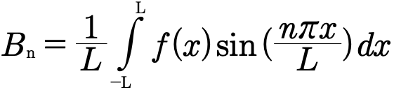
Next substitute in L.
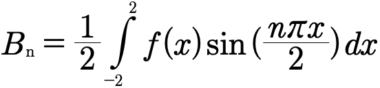
Since  actually has two separate values for different values of x we need to again split up the integral.

The zero again lets us drop one of the terms which can be evaluated pretty easily.

Finally we can use what we solved and plug it all into our series to give us the Fourier Series of  .

When doing Fourier Series knowing your trigonometry inside and out is extremely important since trigonometric functions are in the very definition of the Fourier Series. One particularly useful notion when doing these is that of even and odd functions, it is sometimes very useful to use the idea in order to solve odd integrals or simplify nasty looking expressions.
As I mentioned before Fourier Series are often used in physical sciences and the reason is because they model periodic behavior. In the example we just worked we found an equation which defines something called a square wave. To see this you could look at the definition we used in the beginning and graph by hand or we could graph the series on a computer.
Although graphing by hand would be easy enough to see what’s going on for simple scenarios if we had something more complex using the computer would probably be the best idea. Unfortunately if you stuck this infinite series into a computer it would flip out.
Graphing and Approximating with a Fourier Series
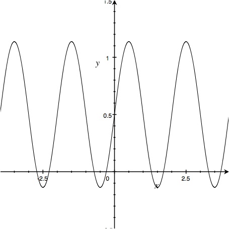
This is the Fourier Series in Example 3.4.1 graphed using only a single term. As you can see it does not look like a square wave.
Read all original image captions
Image 1
This is the Fourier Series in Example 3.4.1 graphed using only a single term. As you can see it does not look like a square wave.
Image 2
The Fourier Series in Example 3.4.1 approximated to 5 terms. Now the fact that this is a square wave is reasonably noticeable but there is still a fair amount of fluctuation at the minimum and maximum values.
Image 3
The Fourier Series in Example 3.4.1 to 100 terms. This is very obviously a square wave and for our purposes of demonstrating the graph of the series is perfect.
Example 3.4.2
Using the function created in example 3.4.1 determine the amount of terms that will properly illustrate that the function created forms a square wave.
Doing something like this generally requires a computer. Writing out even 10 terms of a series is a little difficult let alone 100 or even 1000. That said there are several supplied graphs that will help in this example.
The first graph uses only a single term. As a result of this all we’re looking at is the graph of some slightly modified trigonometric function. Since the goal here was to showcase the fact that this function gives us a square wave and clearly this does not give us anything that would resemble a square wave we will have to use more terms.
The second graph we are given begins to showcase the behavior we are looking for though there is a slight kink. The tops of the wave are fluctuating and are not very flat as you would expect from a square wave so we will up the term by quite a bit more.
The third graph finally gives us what we’re looking for. The tops are essentially flat and give us the square wave form we were looking for.
As you may have noticed in the final graph the square wave has a piece which jumps beyond other pieces at the end. This is a common feature in the Fourier Series at a discontinuity and is called the Gibbs Phenomenon.
Chapter 3 Problems
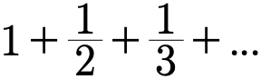
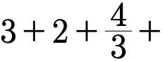
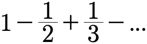
- Determine the type of each of the following series.
- Clarified pattern: (terms for ).
Clarification for part (a): this web edition explicitly uses 1/2−1/3+1/4−… . The source’s displayed 1/2−1/3+1/3−… does not specify an unambiguous continuation. Parts (b)–(e) retain their source expressions.

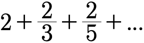
- Determine if the following series are convergent or divergent.

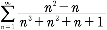
- Use partial fraction decomposition to determine if the following series is telescopic.
- Determine the value of the following series to the 30th term.
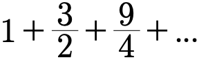

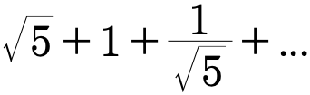
- Determine the value of the following series to an infinite number of terms.
- Create Fourier Series for the following periodic functions.


Glossary and deeper reading · 3 refreshers
These editorial refreshers supplement the reading. Definitions and examples are added guidance; original source wording and recorded answers remain in their original context.
-
Infinite series
An infinite series is the sum of the terms of an infinite sequence, defined through its partial sums. The series converges when those partial sums approach a finite value. For example, 1/2+1/4+1/8+⋯ converges to 1. Terms approaching 0 are necessary for convergence, but that condition alone is insufficient.
-
Interval
An interval is a set of real numbers containing every number between any two of its members. Parentheses exclude an endpoint, while square brackets include it. For example, (1,4] includes 4 and every number between 1 and 4, but excludes 1. An infinite endpoint always uses a parenthesis because infinity is not a real endpoint.
-
Period of a function
A positive period of a function is an input shift that leaves all its outputs unchanged. The fundamental period is the smallest such positive shift when one exists. For example, sin x has fundamental period 2π, while sin(2x) has fundamental period π. The period describes repetition along the input axis rather than the height of an oscillation.