Partial Fractions
This original textbook reading covers part of the AP topic. Follow the AP course outline for complete topic instruction and practice.
Section Overview
- Synthetic Division
- Partial Fractions
- Integrating using Partial Fractions
Section 3
Partial Fractions
Solving integrals by partial fractions looks much more difficult than it actually is. In the end all the method really calls for you to do is solve a system of equations created using a few methods presented in this section and then integrate the equations we create. To get to that point though we will need to recall a skill from algebra.
Synthetic division is something that’s not often used, but it’s incredibly important when solving integrals by partial fractions since you will often be given a large equation to solve which needs to first be reduced. If you recall synthetic division was used to divide two polynomials in the form
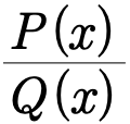
when the degree of  is greater or equal to the degree of
 . The process of synthetic division is best illustrated in an example.
A slightly more visual solution to Example 1.3.1
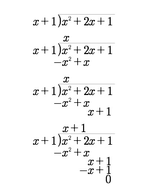
The steps in the text of Example 1.3.1 and this solution are the same. This solution should give a better look at what’s going on though.
Read all original image captions
Image 1
The steps in the text of Example 1.3.1 and this solution are the same. This solution should give a better look at what’s going on though.
Example 1.3.1
Use synthetic division to complete the following operation
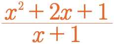
When using synthetic division the first thing you will want to is look at the first terms in both numerator and denominator, these will be divided.
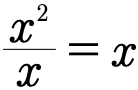
Since we received an  from the division it will be the first term of our answer.
The next thing we must do is take that and multiply our denominator 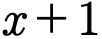 by it.
Therefore

Next take that answer and subtract it from the numerator

We are now left with a new, reduced equation combining our original  , our denominator
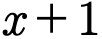 , and the equation from our subtraction .

The last fraction can finally easily be divided to show that
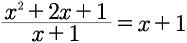
The above process of synthetic division can be repeated until something similar to the second to last equation is reached where one can easily divide or is left with a remainder.
When using partial fractions to integrate we will always concern ourselves with the remainder
The main idea when dealing with partial fractions is to take some fraction with a factored denominator and break it apart into separate fractions. The separate fractions will have different types of numerators and denominators depending on the nature of the original fraction. In the end you will have something similar to this.

You will solve for the constants  ,
 , etc. by multiply everything by the denominator of the left equation.


After rearranging everything we can then set up a system of equations by doing something called equating coefficients.


Equating coefficients is nothing but setting coefficients in a polynomial equal to one another. In this case we may set all coefficients besides the last to zero because on the left side we only have a single term.

so

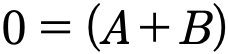
and
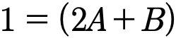
As a shortcut you can skip the portion of this with the x’s and head straight for the coefficients, the x’s were here only to demonstrate the technique.
The system of equations formed by
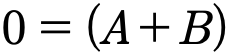 and
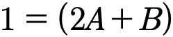
can then be solved using any method you wish giving you the values for  and
 .
The basic techniques used in the previous demonstration will be used in all partial fractions problems different denominators will require you do set up different equations though. The demonstration used only non-repeating linear factors.
For every non-repeating linear factor in a problem you will need to create a single, corresponding fraction which has a constant as a numerator like so

For repeating linear factors you will create fractions whose denominators are the factor but which have an increasing exponent ( look closely at the example since this can be somewhat confusing ).

For prime quadratic factor you will want create fractions with linear numerators as follows.

And finally for prime repeating quadratic factors we will do the following.

Example 1.3.2
Use partial fractions to decompose
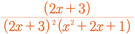
The first thing that must be done in this problem is to simplify the fraction. Looking closely we can see that both a factor of 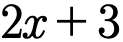 can be taken out and that the quadratic
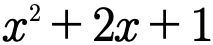 can be reduced.
So since

and
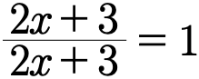
then

Noticing that be have both repeating and non-repeating linear factors this means that

Multiplying through with the left hand denominator gives

Multiplying everything out and rearranging leaves us with

Which by equating coefficients leaves us with the system of equations



Solving this system of equations leaves us with the following values
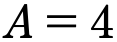
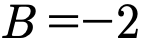
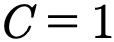
By plugging in these values we get our solution
The final example that I will show you is one in which you will finally use partial fractions to integrate. The process will be the same as the previous example but we will instead at the end deal with the integral.
Example 1.3.3
Integrate the following
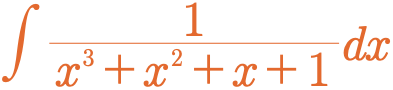
The first thing to realize in this problem is that the polynomial in the denominator can be broken up into two factors.

After this the next thing to notice is that we have a single linear and a single prime quadratic factor in our denominator so that the integrand can be broken up into two terms using the rules for partial fractions.

Looking only at only the insides of the integrals now we can follow the process to figure out the values for  ,
 , and
 .




By equating coefficients we can then create our system of equations.
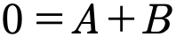
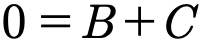
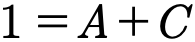
Which by solving through any method gives us the follow values for our coefficients.
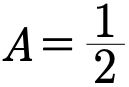 ,
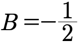 ,
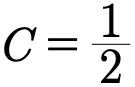
By plugging in these values into our integral we can get a new equation.

Through a couple of algebraic moves we can get something a bit more workable.
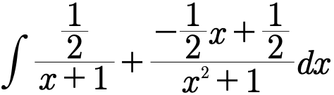


Finally left something we can use we take the needed integrals.



Which added up and with out constant of integration give us our final answer.

Pop Quiz 1.3.1 Partial Fractions
Question 1 of 5 · 0 correct
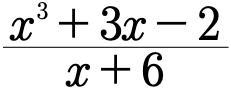
Use synthetic division to solve the follow expression.
Glossary and deeper reading · 2 refreshers
These editorial refreshers supplement the reading. Definitions and examples are added guidance; original source wording and recorded answers remain in their original context.
-
Partial fractions
Partial fraction decomposition writes a rational expression as a sum of simpler fractions. If the numerator’s degree is at least the denominator’s, polynomial division comes first. For example, 1/[x(x+1)] equals 1/x−1/(x+1) wherever the original expression is defined. The factor types and any repeated factors determine the form of the decomposition.
-
Polynomial
A polynomial in one variable is a finite sum of constant multiples of nonnegative integer powers of that variable. The degree is the highest exponent with a nonzero coefficient. For example, 2x³−x+5 is a polynomial of degree 3. Expressions containing 1/x or √x are not polynomials in x.