FFR - Estimating Areas
This original textbook reading covers part of the AP topic. Follow the AP course outline for complete topic instruction and practice.
This reading includes verified answer corrections and explicitly stated clarifications.
For the longest time, there were two separate branches of calculus. The first was derivative calculus, where mathematicians estimated slopes of tangent lines using limits, and there was integral calculus, where mathematicians used limits to estimate areas under curves. Whichever branch you choose, the foundation of Calculus is based on limits.
Using integral calculus, we can set up the area under the curve as small, differential areas (differential just means really really thin). For the sake of simplicity, let’s make these areas rectangular. That way, we only have to worry about length and width. We can also use other shapes for estimating areas, but their calculations are more complicated.
This is going to be a relatively short section, but with lots of pictures to develop a conceptual framework.
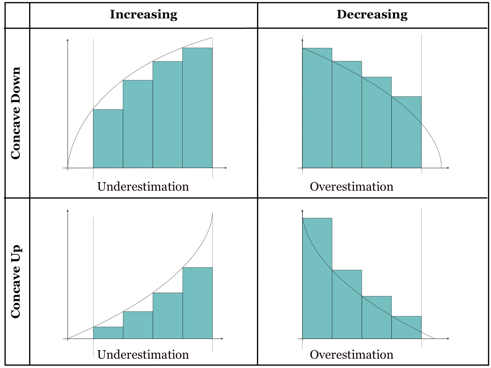
Gallery 6.4.1 Estimation accuracy using different methods of Approximation
Read all original image captions
Image 1
Image 2
Image 3
For a function that is concave up throughout the interval, midpoint sums underestimate the definite integral. Concave down throughout gives an overestimate. The sketches show the direction of the error; the word “slight” in an image is not a general error bound. The size depends on the function and partition.
Image 4
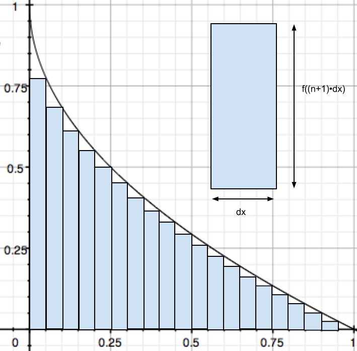
Interactive 6.4.1 The best way to estimate
Read all original figure notes
Rectangle width Δx
As Δx approaches 0
Example Problem 6.4.1
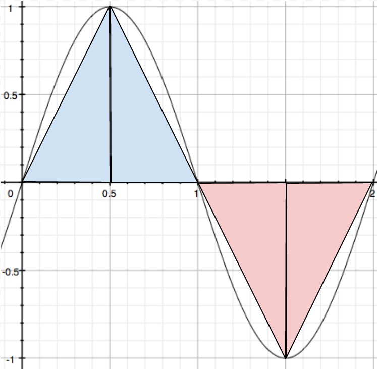
Using the trapezoids method, estimate the area under the curve of from x = 0 to x = 2, with n, the number of trapezoids, equal to 4.
Interactive 6.4.2 Understanding trapezoidal areas
Read all original figure notes
The vertical sides
dx
Triangle?
Signed accumulation and area
Show your work for Problem 1
Clarification: Use the asset model . Here the given r(t) is inserted into the exponent t r(t); it is not an instantaneous proportional growth rate.
Drawing is temporarily unavailable. Work on paper if needed, then record your reasoning here.
Saving written working requires JavaScript. Keep your work on paper or in your own notes; the source problem above remains available.
- You open up a business using $10 000 of your hard-earned money. You think that the rate of return on your investment (as a decimal) can be modeled by the equation . What is the rate of increase of the assets in your business after 3 years? Use units of dollars per year.
Clarification: Use the asset model . Here the given r(t) is inserted into the exponent t r(t); it is not an instantaneous proportional growth rate.
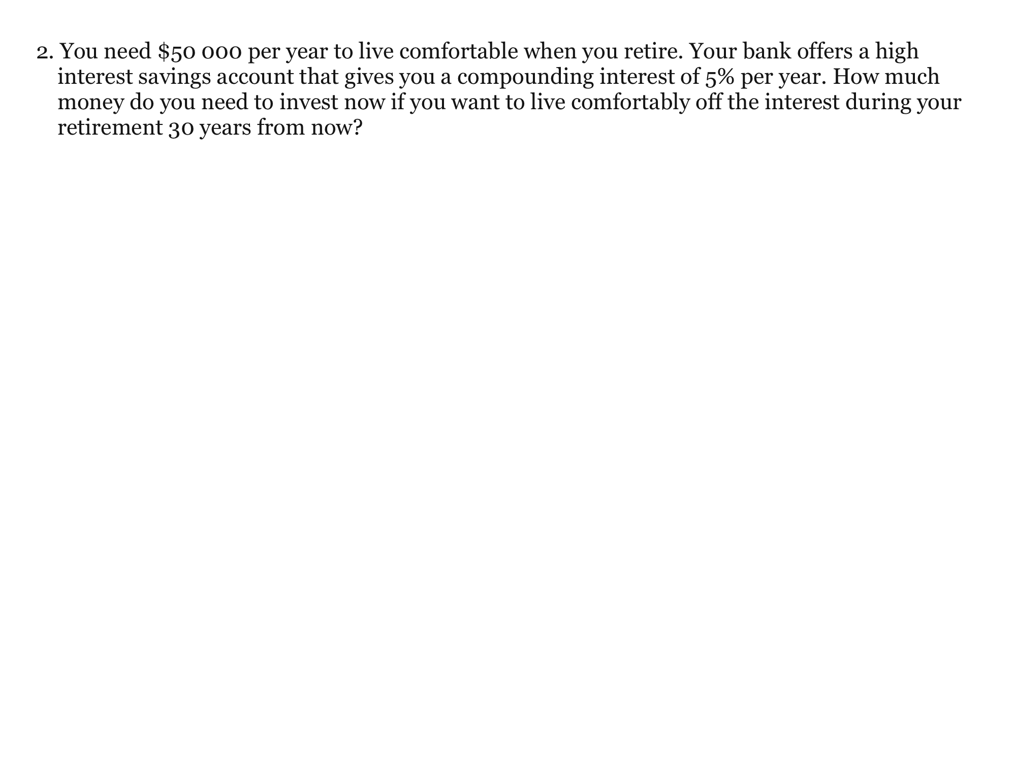
- You need $50 000 per year to live comfortably when you retire. Your bank offers a high interest savings account that gives you a compounding interest of 5% per year. How much money do you need to invest now if you want to live comfortably off the interest during your retirement 30 years from now ?
Clarification: Assume continuous compounding. The retirement fund is chosen so that interest at 5% supplies $50,000 per year without using the principal.
Show your work for Problem 2
Clarification: Assume continuous compounding. The retirement fund is chosen so that interest at 5% supplies $50,000 per year without using the principal.
Drawing is temporarily unavailable. Work on paper if needed, then record your reasoning here.
Saving written working requires JavaScript. Keep your work on paper or in your own notes; the source problem above remains available.
Show your work for Problem 4
a) What is the optimum number of laptops your company should make for profit maximization?
b) What is the annual profit at that quantity?
Drawing is temporarily unavailable. Work on paper if needed, then record your reasoning here.
Saving written working requires JavaScript. Keep your work on paper or in your own notes; the source problem above remains available.
Show your work for Problem 3
a) What is the optimum price point?
b) How many units will you sell at this price?
Drawing is temporarily unavailable. Work on paper if needed, then record your reasoning here.
Saving written working requires JavaScript. Keep your work on paper or in your own notes; the source problem above remains available.
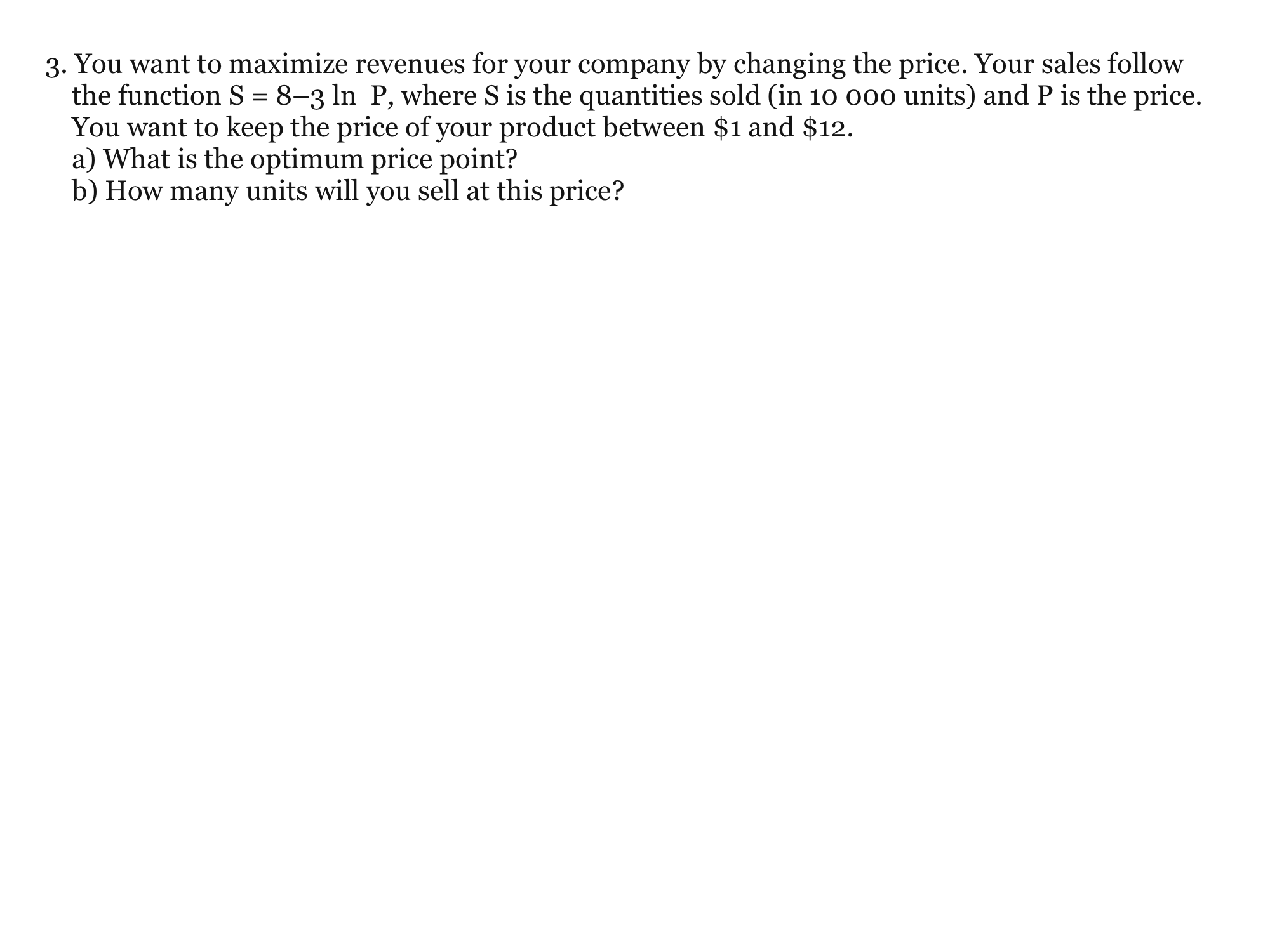
- You want to maximize revenues for your company by changing the price. Your sales follow the function , where S is the quantities sold (in 10 000 units) and P is the price. You want to keep the price of your product between $1 and $12.
a) What is the optimum price point?
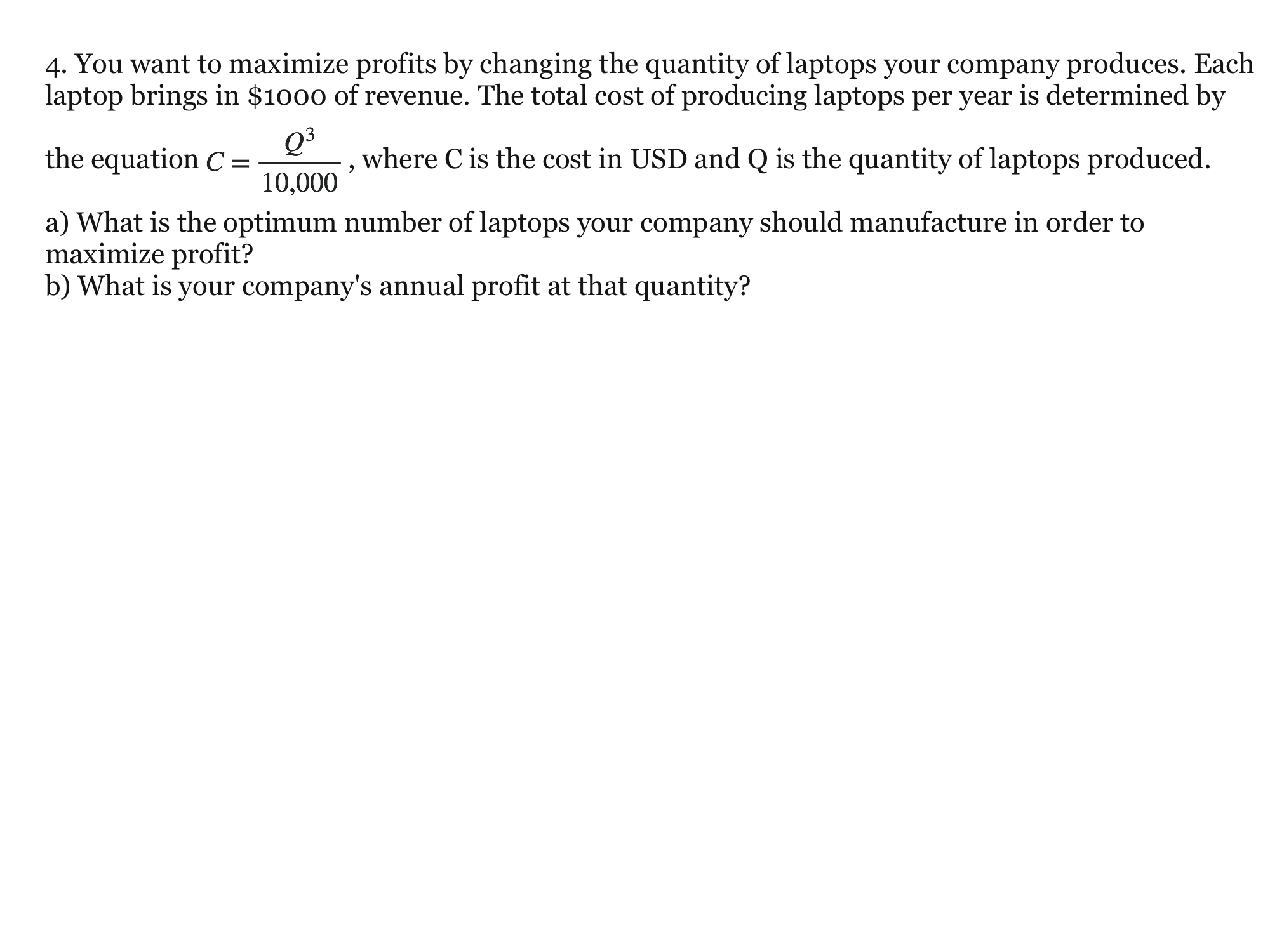
b) How many units will you sell at this price? - You want to maximize profits by changing the quantity of laptops your company produces. Each laptop brings in $1000 of revenue. The total cost of producing laptops per year is represented by , where C is the cost and Q is the quantity of laptops produced.
a) What is the optimum number of laptops your company should make for profit maximization?
b) What is the annual profit at that quantity?
Show your work for Problem 5
Drawing is temporarily unavailable. Work on paper if needed, then record your reasoning here.
Saving written working requires JavaScript. Keep your work on paper or in your own notes; the source problem above remains available.
Show your work for Problem 6
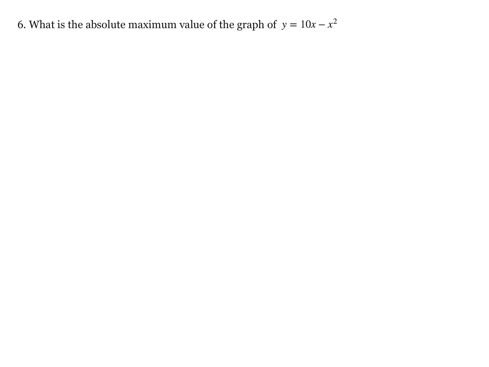
Drawing is temporarily unavailable. Work on paper if needed, then record your reasoning here.
Saving written working requires JavaScript. Keep your work on paper or in your own notes; the source problem above remains available.
Show your work for Problem 7
a) At which point does its absolute maximum value occur?
b) What is the maximum value?
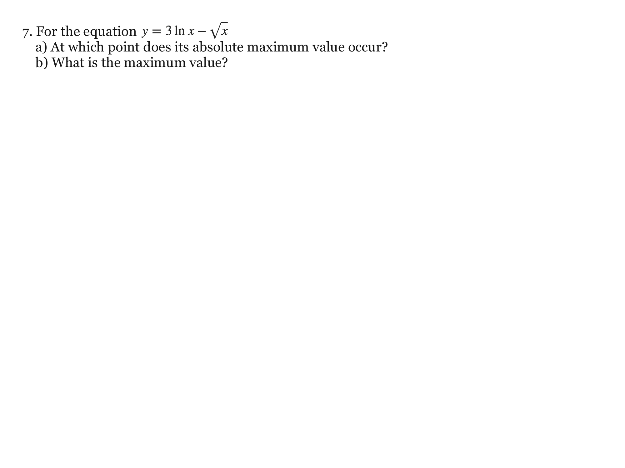
Drawing is temporarily unavailable. Work on paper if needed, then record your reasoning here.
Saving written working requires JavaScript. Keep your work on paper or in your own notes; the source problem above remains available.
Show your work for Problem 8
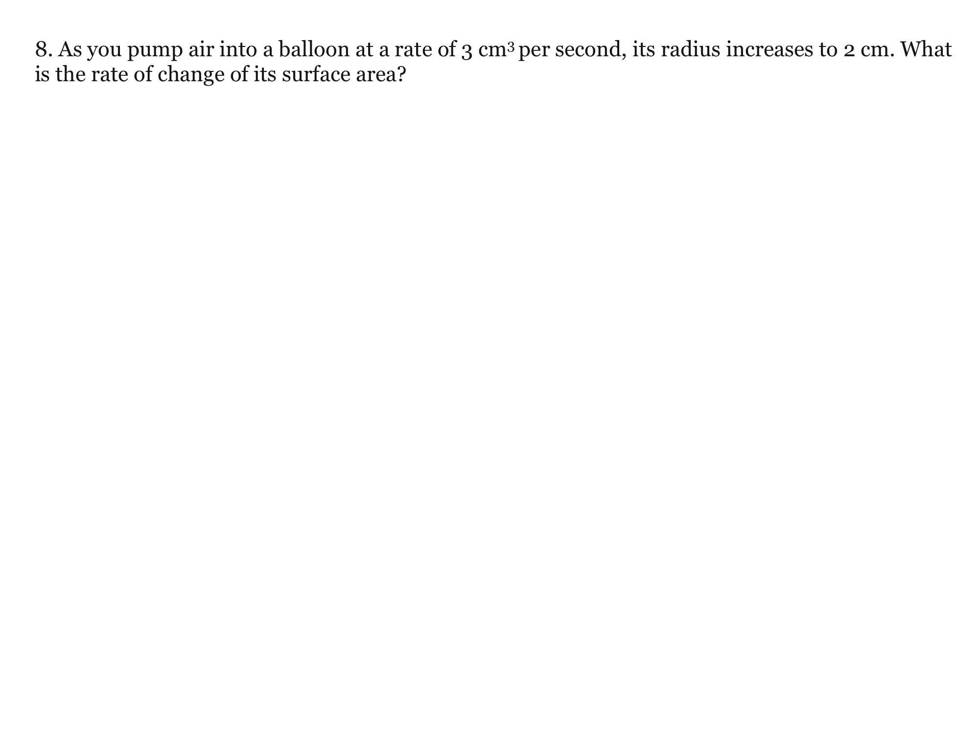
Drawing is temporarily unavailable. Work on paper if needed, then record your reasoning here.
Saving written working requires JavaScript. Keep your work on paper or in your own notes; the source problem above remains available.
Show your work for Problem 9
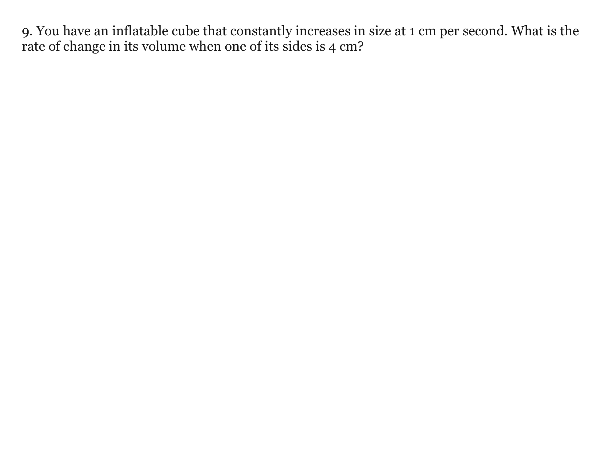
Drawing is temporarily unavailable. Work on paper if needed, then record your reasoning here.
Saving written working requires JavaScript. Keep your work on paper or in your own notes; the source problem above remains available.
Show your work for Problem 10
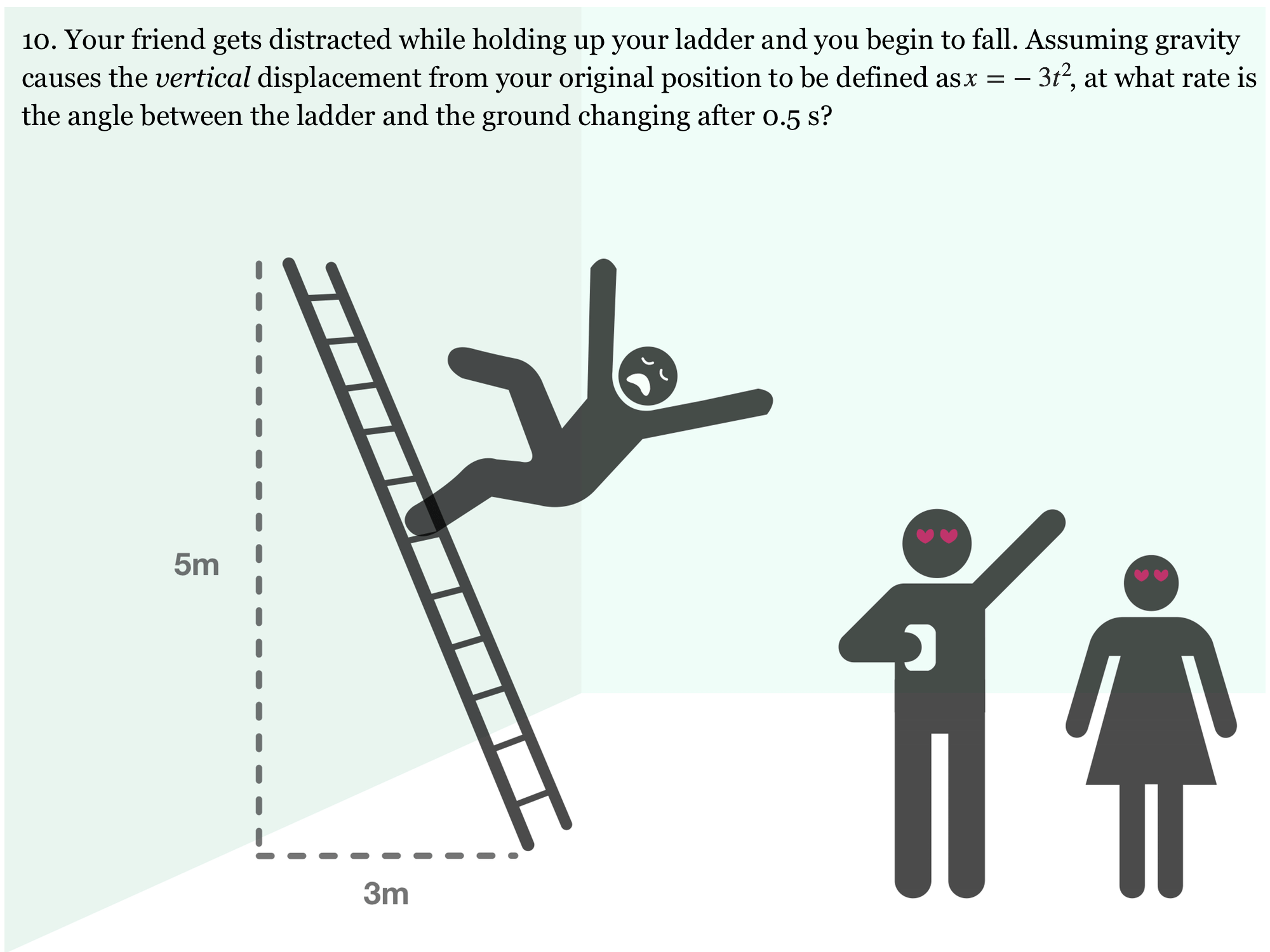
Clarification: Treat the ladder as rigid, with its foot sliding on horizontal ground. Use the source diagram’s initial height 5 m and base distance 3 m; the top height is 5−3t² metres.
Drawing is temporarily unavailable. Work on paper if needed, then record your reasoning here.
Saving written working requires JavaScript. Keep your work on paper or in your own notes; the source problem above remains available.
- You have an inflatable cube that constantly increases in size at 1cm per second. What is the rate of change in its volume when one of its sides is 4 cm?
- Your friend gets distracted while holding up your ladder and you feel yourself starting to fall. Assuming gravity causes the vertical displacement from your original position to be defined as , at what rate is the angle between the ladder and the ground changing after 0.5s?
Clarification: Treat the ladder as rigid, with its foot sliding on horizontal ground. Use the source diagram’s initial height 5 m and base distance 3 m; the top height is 5−3t² metres.
Glossary and deeper reading · 2 refreshers
These editorial refreshers supplement the reading. Definitions and examples are added guidance; original source wording and recorded answers remain in their original context.
-
Integral
Integration can mean accumulating a function over an interval or finding an antiderivative. A definite integral gives a number, while an indefinite integral represents a family of antiderivatives. For example, integrating 2x indefinitely gives x²+C, and integrating it from 0 to 2 gives 4. The Fundamental Theorem of Calculus connects these two operations under its hypotheses.
-
Differential
For a differentiable function y=f(x), the differential dy is defined as f′(x) dx. It represents the tangent-line estimate of the output change associated with an input change dx. For example, y=x² at x=3 and dx=0.01 gives dy=6·0.01=0.06. The actual change in y can differ from this linear estimate.