Approximation and Second Derivatives
This original textbook reading covers part of the AP topic. Follow the AP course outline for complete topic instruction and practice.
This reading includes verified answer corrections and explicitly stated clarifications.
Interactive 3.3.1 Newton-Raphson Method
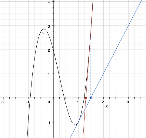
Read all original figure notes
3) Next iteration
1) The initial guess
2) The Approximation
Often we are interested in finding the roots (or zeros) of a function, but we do not want to do all that work, so we ask a computer to do it for us. The problem? Computers cannot solve equations. So we have to provide them with the steps to come up with an approximate solution. Here is one method:
Moving from the initial guess to the next x-value can be accomplished by using the formula:
A closer examination reveals that this is simply the original formula of a derivative/slope rearranged!
We use a 0 here because we are interested in the roots of the function, or when it crosses y = 0. This is our .
We can test to see that the formula is true by referring to the graph on the previous page. With an initial guess of 1, the slope of the tangent line at that point was equal to 2, and the function value at 1 was equal to -1. Plugging those values into the equation gives
or 1.5, which as it turns out, is the point at which the blue tangent line crosses the x-axis! Let’s try our hand at some problems using the Newton-Raphson Method.
Example Problem 3.3.1
Compute two iterations to get a numerical approximation of the root of the function starting at x = 2.
Note: Notice that we reach the second iteration when x’s value is 3, or 1 greater than our desired number of iterations. This is why sometimes the Newton-Raphson formula is written as
.
Limitations of the Newton-Raphson Method
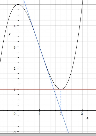
The Newton Raphson Method often only works when the initial guess is close to the solution. Otherwise, we could run into a few inconveniences, as shown in Gallery 3.3.1. So remember, make a good initial guess.
Gallery 3.3.1 Inconveniences related to Newton-Raphson
Read all original image captions
Image 1
Image 2
Glossary and deeper reading · 3 refreshers
These editorial refreshers supplement the reading. Definitions and examples are added guidance; original source wording and recorded answers remain in their original context.
-
Derivative
A derivative gives the instantaneous rate of change of a function with respect to its input. At a point, it is the finite limit of the difference quotient when that limit exists. For example, the derivative of x² is 2x, so the tangent slope at x=3 is 6. A derivative function collects those rates across the inputs where the function is differentiable.
-
Tangent line
A tangent line at a differentiable point passes through the point and has slope equal to the derivative there. It describes the function’s local linear behavior. For example, y=x² has tangent line y=4+4(x−2) at x=2. A tangent can cross the curve, so touching at exactly one point is not its general definition.
-
Function
A mathematical function assigns exactly one output to each input in its domain. Inputs can share an output, but one input cannot have two different outputs. For example, f(x)=x² assigns the output 9 to both 3 and −3. Function notation names the rule and its input; f(3) means the output when the input is 3.