Differentiability

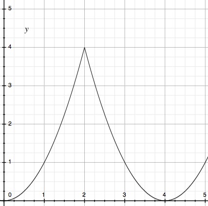
When is a function differentiable?

A function is differentiable at a point exactly when its difference quotient has a finite two-sided limit: lim_h→0 [f(a + h) − f(a)]/h. The following are useful warning signs, not a complete checklist proving differentiability.

• Differentiability implies continuity. Continuity by itself does not imply differentiability: |x| is continuous at 0 but has different one-sided slopes.
• Corners and cusps can prevent a derivative. At a corner the finite one-sided derivatives differ; at a cusp a finite two-sided derivative also fails. Always test the limiting slopes.
• A vertical tangent does not give a finite derivative. Oscillation can also prevent the derivative: let f(x) = x sin(1/x) for x ≠ 0 and f(0) = 0. It is continuous at 0, but its difference quotient sin(1/h) has no limit. A picture alone cannot certify differentiability.

Notation

So far we have seen the derivative of a function written as:

$\underset{h\to 0}{lim}\frac{f(x+h)-f(x)}{h}$ , or in other words $\frac{\mathrm{\Delta }y}{\mathrm{\Delta }x}$ for really, really small changes in y and x. However, ever since we learned to calculate the derivatives of functions in the form of another function (recall Example Problem 2.4.1), it might be inconvenient to write the derivative as a limit over and over again. As a result, mathematicians have come up with many convenient shorthand ways to demonstrate the derivative of a function. Each of these has a slightly different meaning.

Some notations for derivatives

• $dx,dt,dy$ - This notation represents a very small change in or a very small piece of x, t, or y, respectively. This is also known as a differential. Differentials can be functions of each other as well, and have an entire course named after them.
• $\frac{d}{dx},\frac{d}{dy},\frac{d}{dt}$ - These all represent general change with respect to a specific variable. The d can be thought of as delta, except for very small values so that we can distinguish between slope and derivative.
• $\frac{dx}{dt},\frac{dy}{dt},\frac{dy}{dx}$ - These represent change in one variable with respect to another variable. This is what we are usually solving for, with $\frac{dy}{dx}$ being the most common. The notation only varies depending on the variables we choose.
• $\stackrel{·}{x},\stackrel{·}{y}$ - This represents the derivative of the dependent variable in an equation (usually y) with the dependent variable (usually x or t) being implied. This notation is most commonly used in science and engineering problems, where many variables are involved, and it is simplest to show their derivatives with just one or two dots over them (two dots represent second order derivatives).
• $y^{\prime },y^{\prime \prime }$ - pronounced “why prime” and “why double prime” respectively, these are commonly used by mathematicians. The number of primes on a variable represent how many times to take the derivative of the function. Again, the independent variable is implied here.
• $f^{\prime }(x),f^{\prime \prime }(x),f^{\text{n}}(x)$ - This notation is convenient for representing higher order derivatives and eventually generalizing formulas for the “nth” derivative. Sometimes the independent variable is implied and the notation changes to f’, f’’, f’’’, etc.

Example Problem 3.1.1

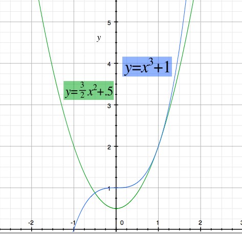
If it exists, find the derivative at x=1 of the piece-wise function:​
$f(x)=\{\begin{array}{rlr}{x}^3+1& \phantom{p}if& x<1\\ \frac{3x^2+1}{2}& \phantom{p}if& x\ge 1\end{array}$

Motivation: Get ready, because this will likely be one of the most challenging example problems you have encountered so far. So challenging, in fact, that I almost did not want to put this in here. However, if you can learn how to do this problem, you will have mastered the concept behind a derivative. Get set, go!

A shortcut to finding derivatives: The Power Rule

We have learned to calculate a derivative using limits, but this can get troublesome, having to take a limit every time we want to find the derivative. The good news is there is a shortcut called the power rule, which lets us find the derivative of any degree polynomial function (including fractional and negative degrees). The power rule looks something like this:

$\frac{d}{dx}{x}^n=n\cdot x^{n-1}$​
So we can find the derivative of x raised to any power by simply multiplying the function by the power, then reducing the power by 1. The simplest proof of the power rule involves using Pascal’s triangle to expand and write the derivative in a general form using the x approaching a definition of a derivative. You might be interested in trying to prove it independently if you are a mathematics major, but we will skip over it for now.