FFR - Anti-derivatives
This original textbook reading covers part of the AP topic. Follow the AP course outline for complete topic instruction and practice.
This reading includes verified answer corrections and explicitly stated clarifications.
You can think of anti-derivatives as, obviously the opposite of a derivative. Since we are already familiar with many derivatives, we just have to learn to think backwards. For example, what is the anti-derivative of ? This is a simple one.
What about the anti-derivative of ? That is a little trickier. We have to invent something we can call the anti-Power Rule.
Anti-Derivative of a polynomial
If we take the derivative of that, we get the base function, . The idea is just working backwards from derivatives now. You might be wondering how this is helpful at all, or why we are skipping around, but it will all click together in the next chapter.
What is the anti-derivative of at , provided there is no constant in the original function?
By now, we have hopefully become more proficient in taking anti-derivatives. What do they mean, physically though?
I don’t want to give too much away, but anti-derivatives help us find accurate measures of areas under curves.
Show your work for Problem 1
Drawing is temporarily unavailable. Work on paper if needed, then record your reasoning here.
Saving written working requires JavaScript. Keep your work on paper or in your own notes; the source problem above remains available.
Show your work for Problem 2
Drawing is temporarily unavailable. Work on paper if needed, then record your reasoning here.
Saving written working requires JavaScript. Keep your work on paper or in your own notes; the source problem above remains available.
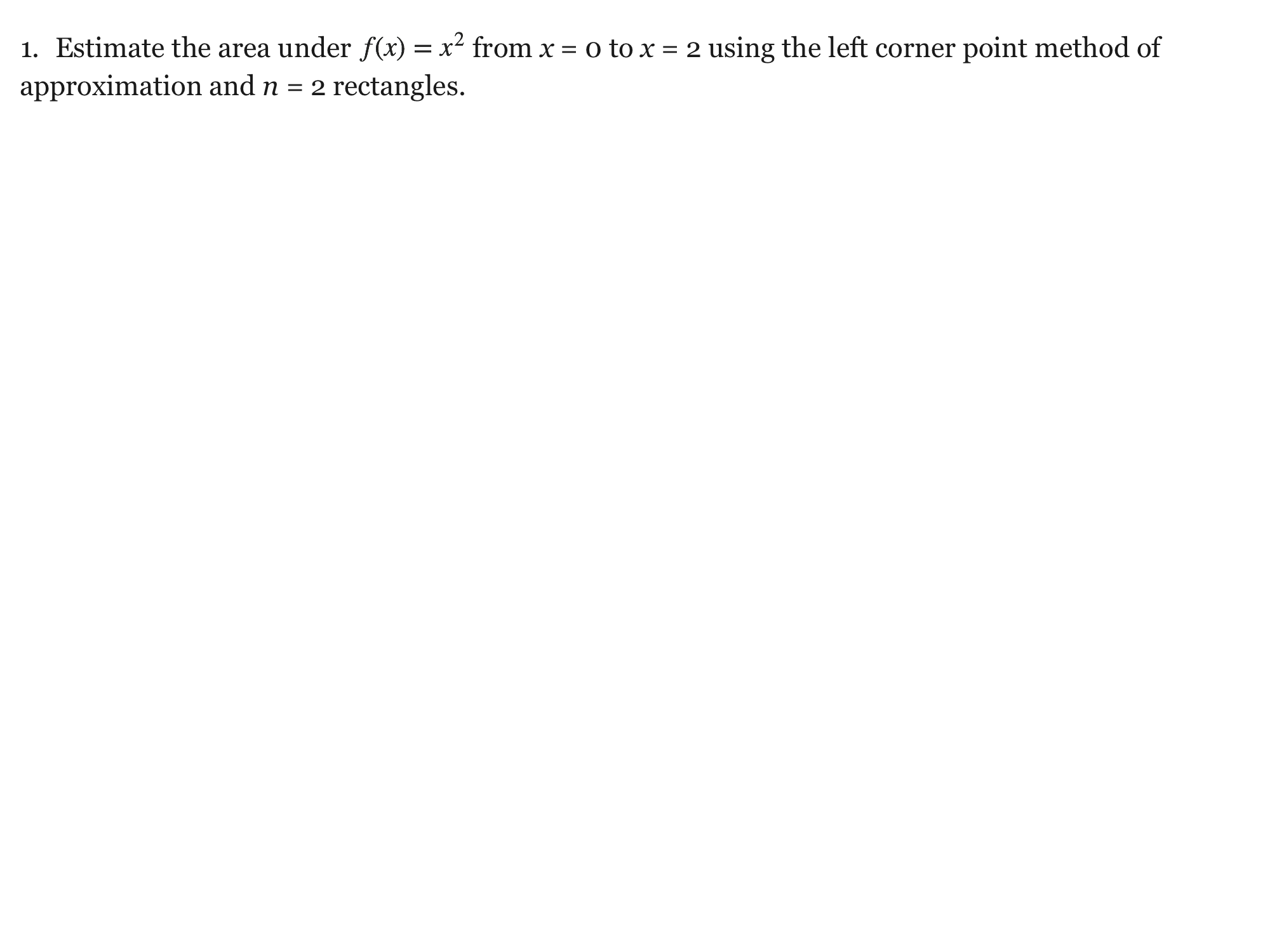
- Estimate the area under from x = 0 to x = 2 using the left corner point method of approximation and n = 2 rectangles.
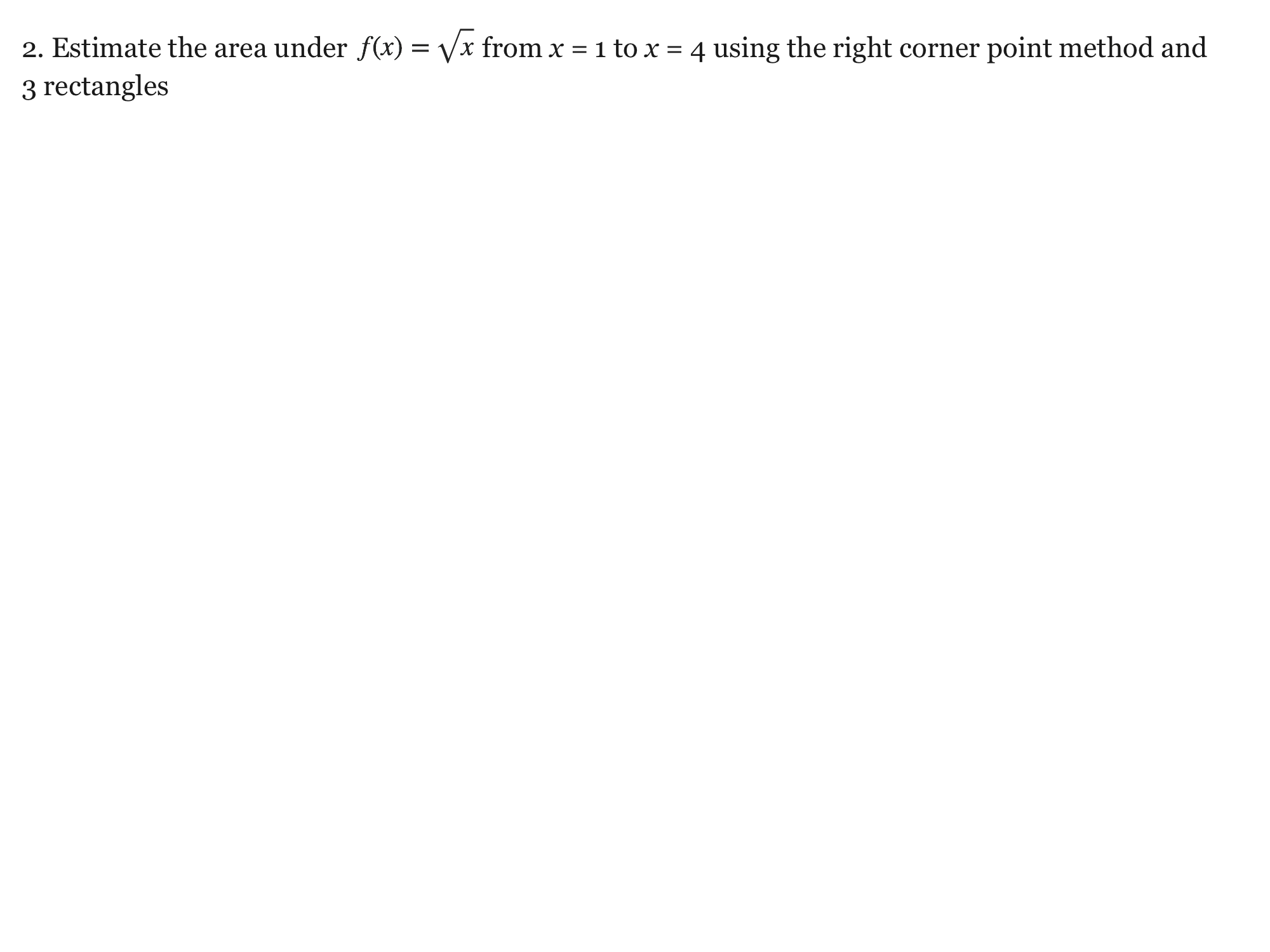
- Estimate the area under from x = 1 to x = 4 using the right corner point method and 3 rectangles.
Show your work for Problem 4
Drawing is temporarily unavailable. Work on paper if needed, then record your reasoning here.
Saving written working requires JavaScript. Keep your work on paper or in your own notes; the source problem above remains available.
Show your work for Problem 3
Drawing is temporarily unavailable. Work on paper if needed, then record your reasoning here.
Saving written working requires JavaScript. Keep your work on paper or in your own notes; the source problem above remains available.
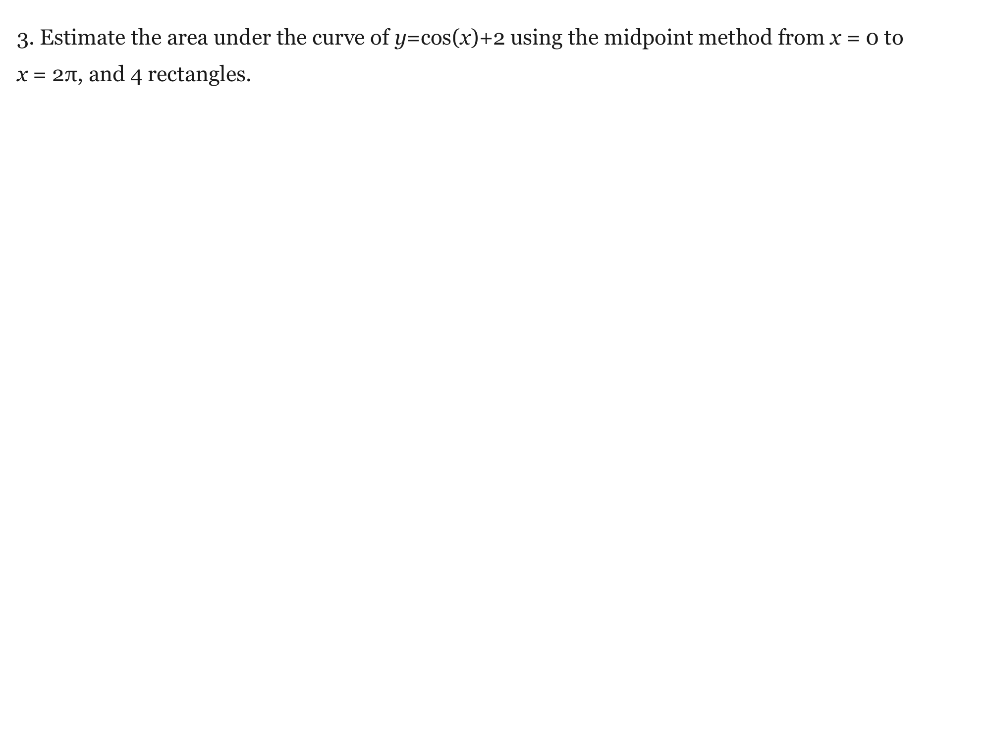
- Estimate the area under the curve of using the midpoint method from x = 0 to x = 2π, and 4 rectangles.
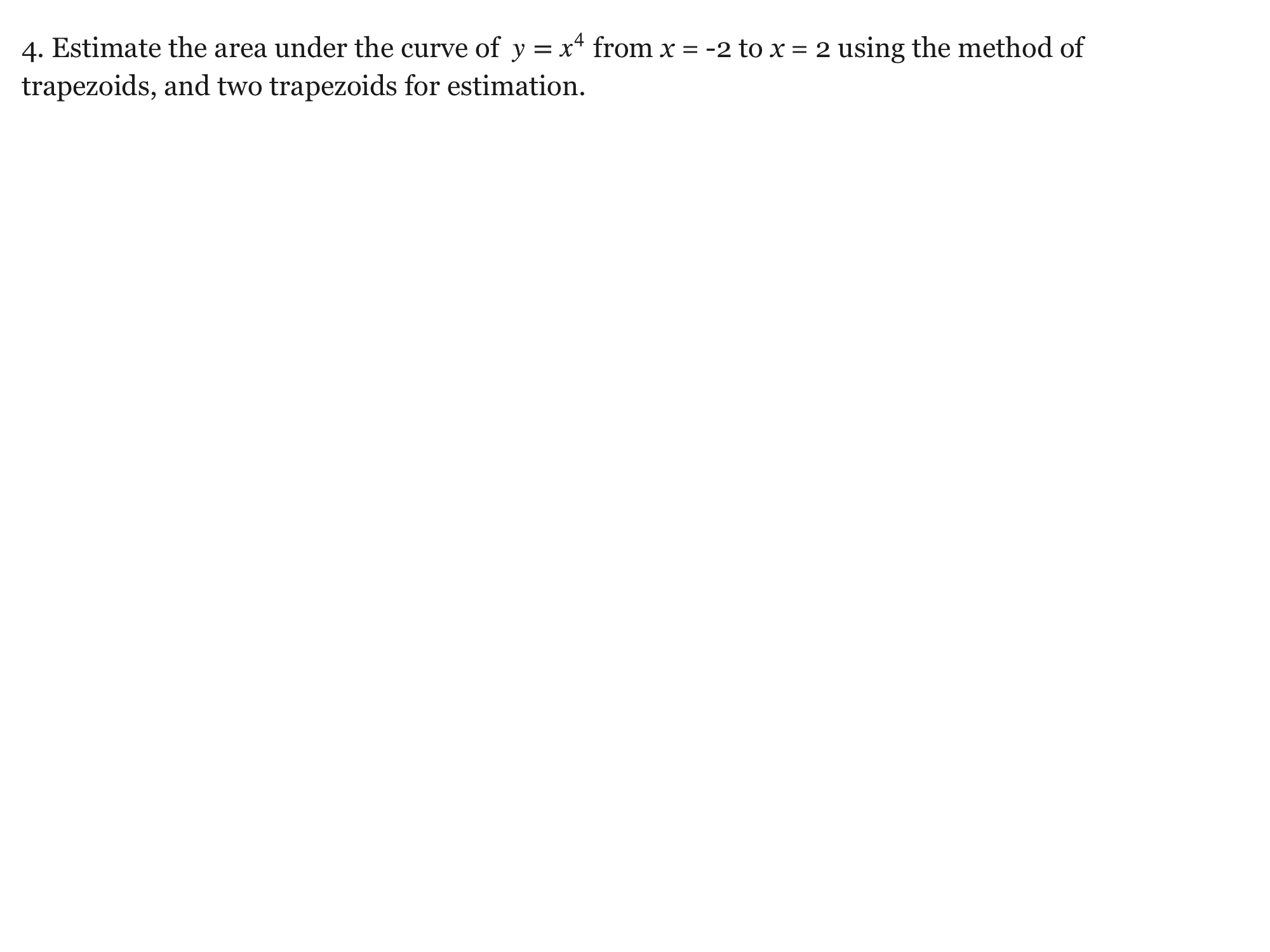
- Estimate the area under the curve of from x = -2 to x = 2 using the method of trapezoids and 2 trapezoids for estimation.
Show your work for Problem 6
Drawing is temporarily unavailable. Work on paper if needed, then record your reasoning here.
Saving written working requires JavaScript. Keep your work on paper or in your own notes; the source problem above remains available.
Show your work for Problem 5
Drawing is temporarily unavailable. Work on paper if needed, then record your reasoning here.
Saving written working requires JavaScript. Keep your work on paper or in your own notes; the source problem above remains available.
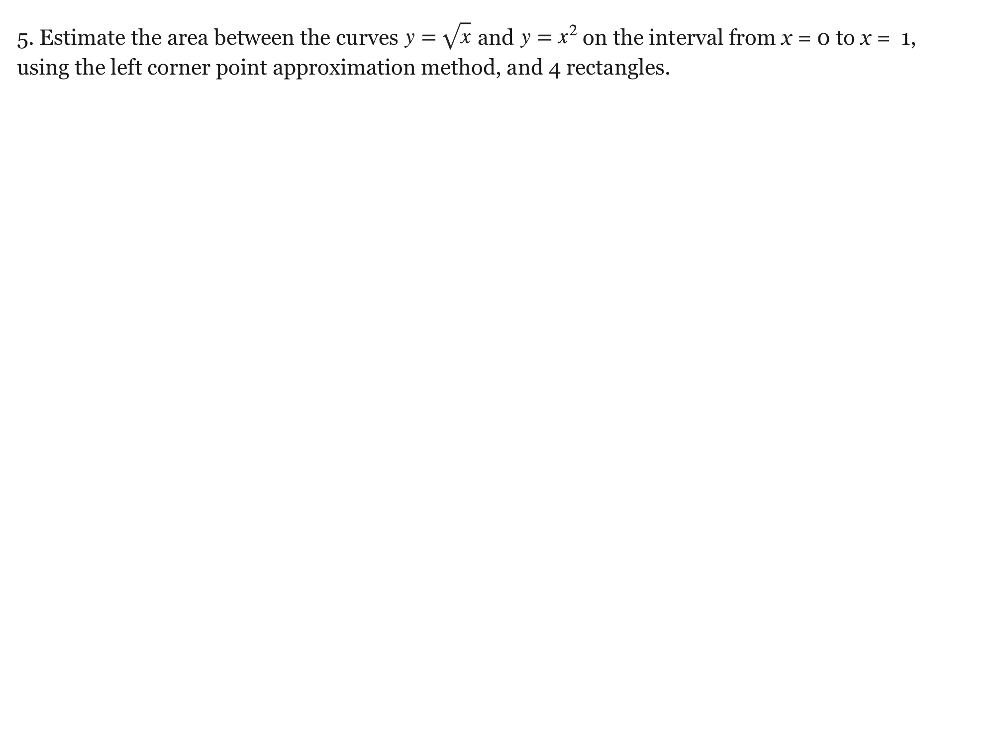
- Estimate the area between the curves and on the interval from x = 0 to x = 1 using the left corner point approximation method and 4 rectangles.
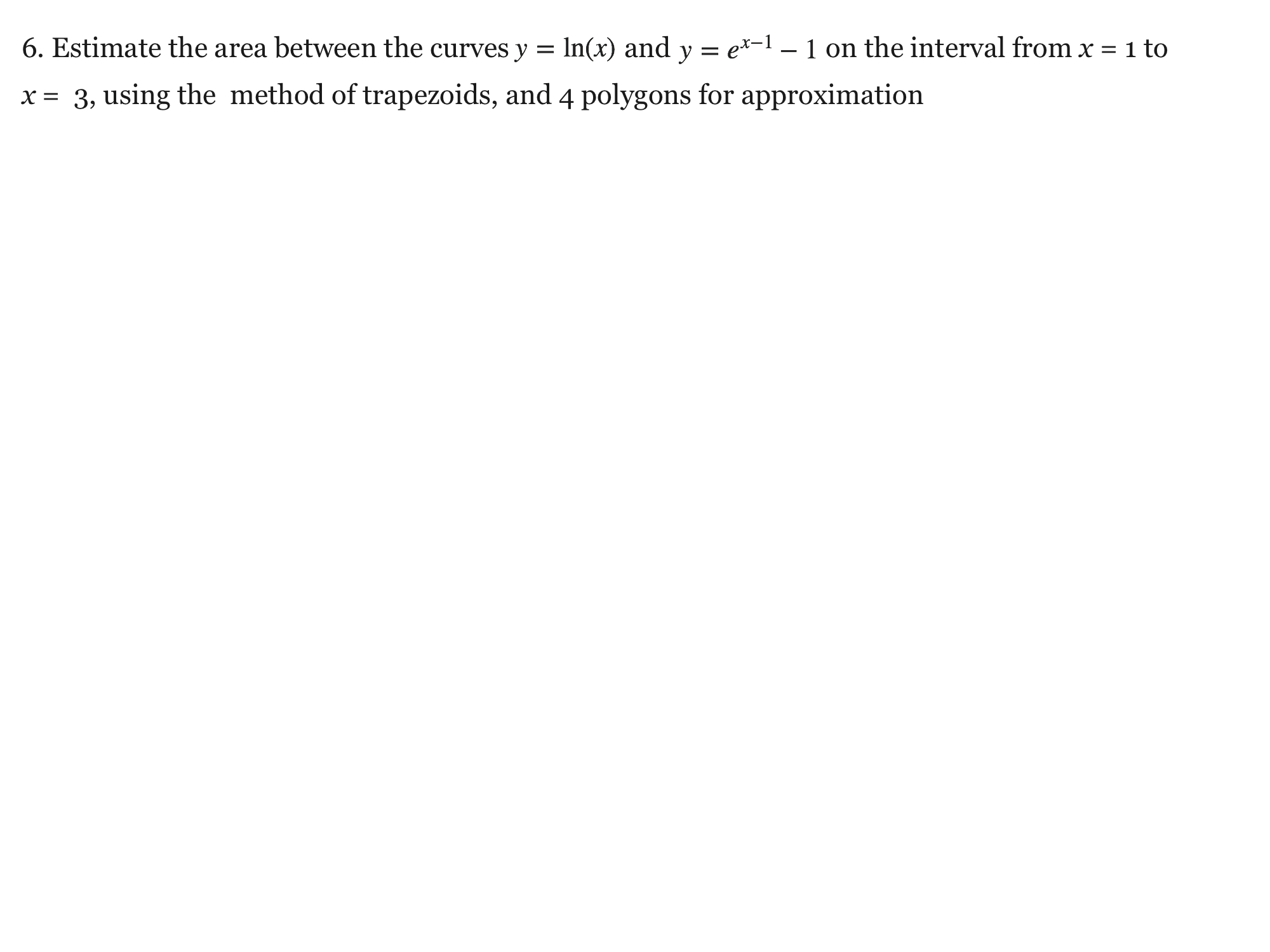
- Estimate the area between the curves and from x = 1 to x = 3 using the method of trapezoids and 4 polygons for approximation.
Show your work for Problem 8
Drawing is temporarily unavailable. Work on paper if needed, then record your reasoning here.
Saving written working requires JavaScript. Keep your work on paper or in your own notes; the source problem above remains available.
Show your work for Problem 7
Clarification: Estimate geometric area between the curve and the x-axis, using the absolute value of each right-endpoint height.
Drawing is temporarily unavailable. Work on paper if needed, then record your reasoning here.
Saving written working requires JavaScript. Keep your work on paper or in your own notes; the source problem above remains available.
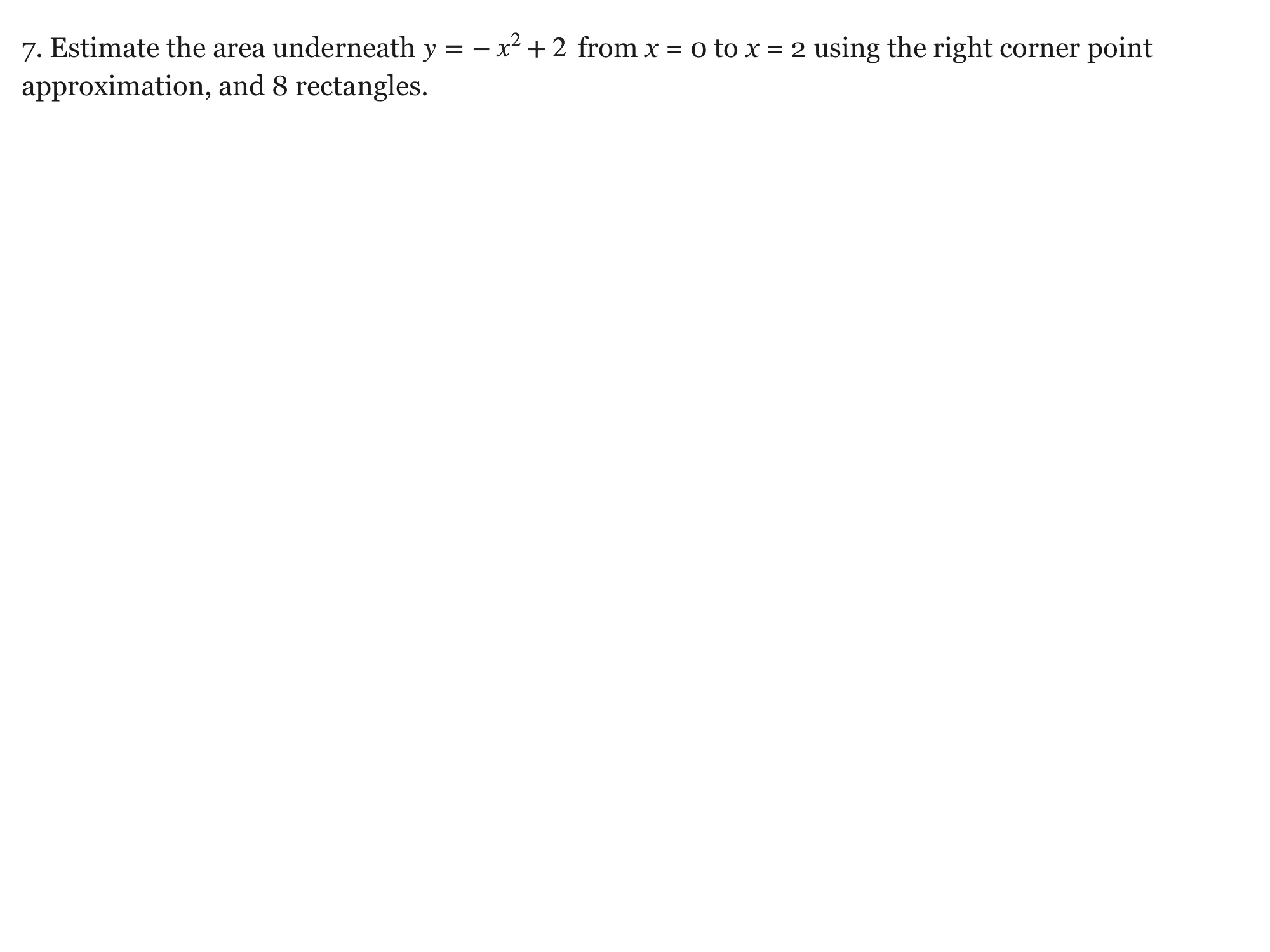
- Estimate the area underneath from x = 0 to x = 2 using right corner point approximation and 8 rectangles.
Clarification: Estimate geometric area between the curve and the x-axis, using the absolute value of each right-endpoint height.
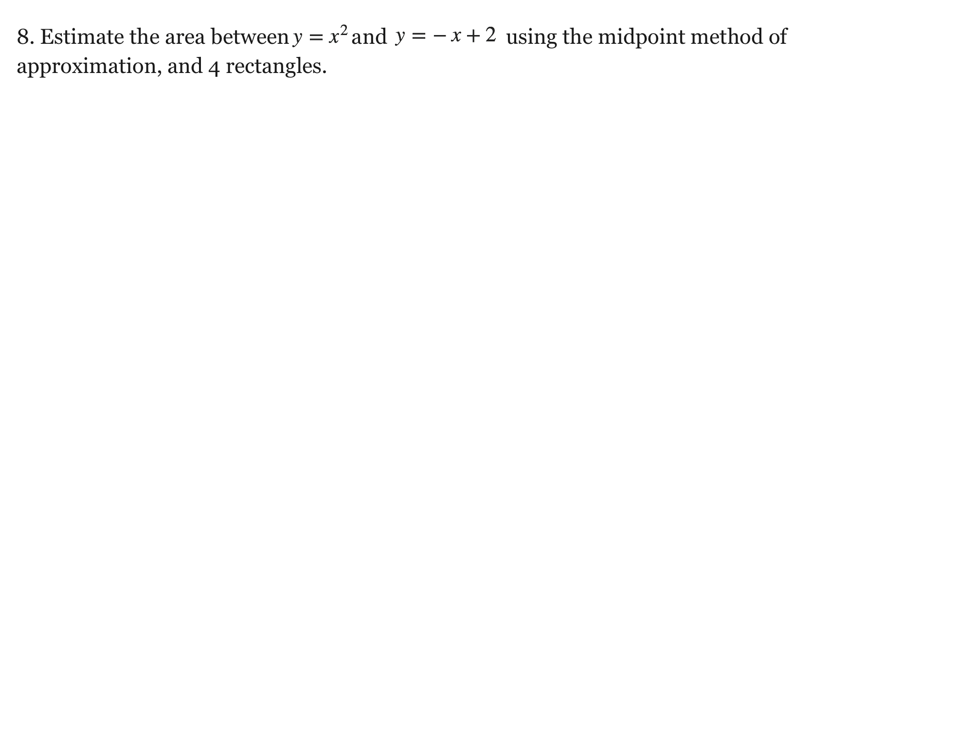
- Estimate the area between and from x = 0 to x = 1 using the midpoint method of approximation and 4 rectangles.
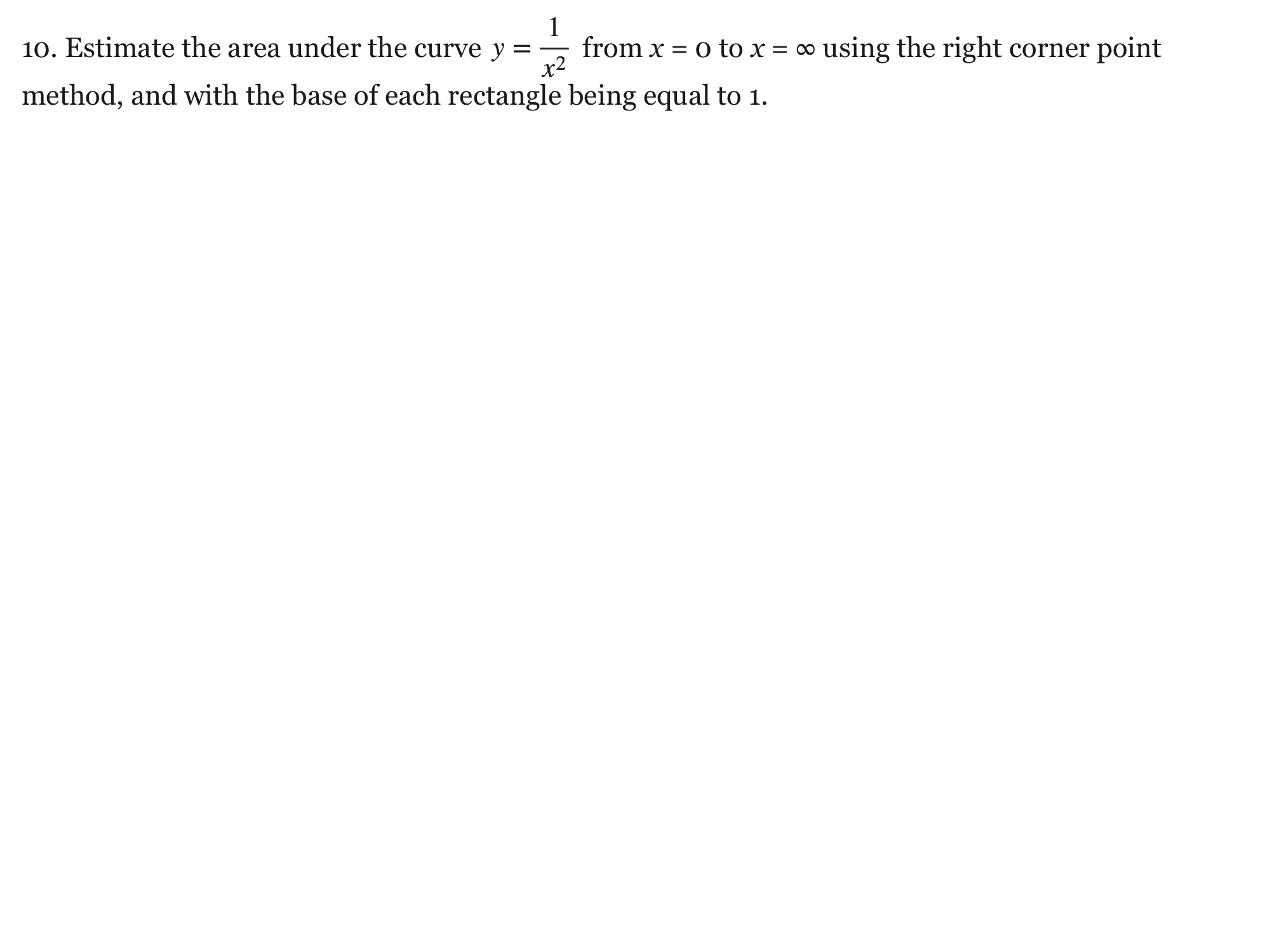
Show your work for Problem 10
Clarification: Estimate the unit-width right-rectangle sum, whose sample points are 1,2,3,… . This is a sampled estimate; the exact improper area starting at x=0 diverges.
Drawing is temporarily unavailable. Work on paper if needed, then record your reasoning here.
Saving written working requires JavaScript. Keep your work on paper or in your own notes; the source problem above remains available.
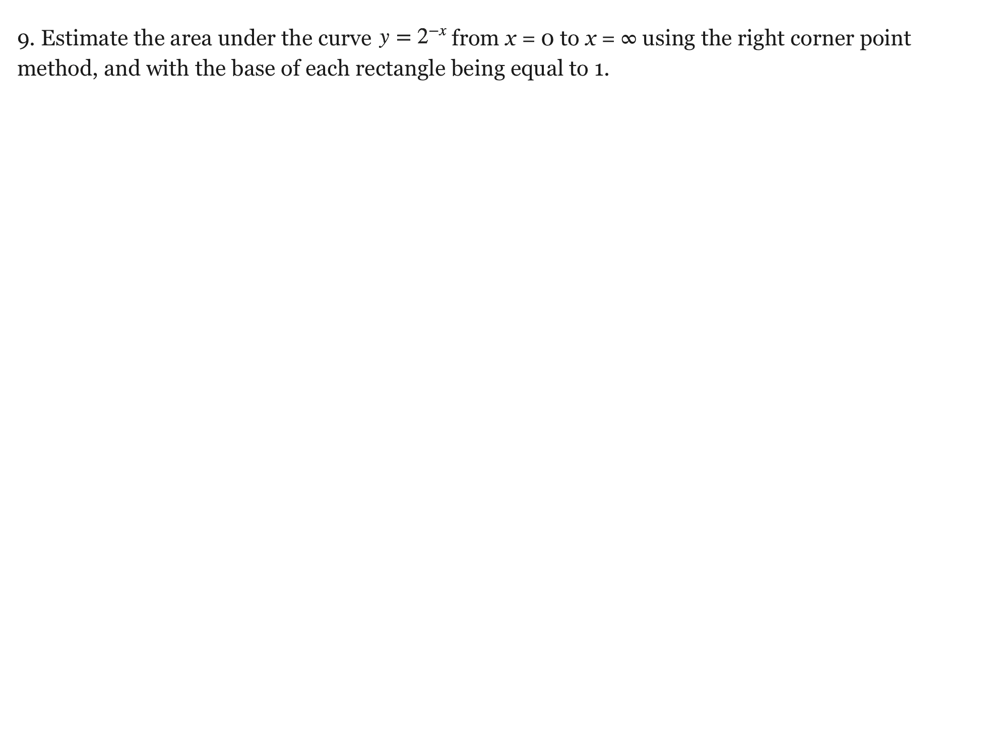
Show your work for Problem 9
Drawing is temporarily unavailable. Work on paper if needed, then record your reasoning here.
Saving written working requires JavaScript. Keep your work on paper or in your own notes; the source problem above remains available.
- Estimate the area under the curve from x = 0 to x = ∞ using the right corner point method and with the base of each rectangle being equal to 1.
- Estimate the area under the curve from x = 0 to x = ∞ using the right corner point method and with the base of each rectangle being equal to 1.
Clarification: Estimate the unit-width right-rectangle sum, whose sample points are 1,2,3,… . This is a sampled estimate; the exact improper area starting at x=0 diverges.
Glossary and deeper reading · 4 refreshers
These editorial refreshers supplement the reading. Definitions and examples are added guidance; original source wording and recorded answers remain in their original context.
-
Derivative
A derivative gives the instantaneous rate of change of a function with respect to its input. At a point, it is the finite limit of the difference quotient when that limit exists. For example, the derivative of x² is 2x, so the tangent slope at x=3 is 6. A derivative function collects those rates across the inputs where the function is differentiable.
-
Antiderivative
An antiderivative of a function is another function whose derivative equals the original function on an interval. Two antiderivatives on the same interval differ by a constant. For example, x² is an antiderivative of 2x, and x²+7 is another. An antiderivative is a function, whereas a definite integral is an accumulated value.
-
Polynomial
A polynomial in one variable is a finite sum of constant multiples of nonnegative integer powers of that variable. The degree is the highest exponent with a nonzero coefficient. For example, 2x³−x+5 is a polynomial of degree 3. Expressions containing 1/x or √x are not polynomials in x.
-
Function
A mathematical function assigns exactly one output to each input in its domain. Inputs can share an output, but one input cannot have two different outputs. For example, f(x)=x² assigns the output 9 to both 3 and −3. Function notation names the rule and its input; f(3) means the output when the input is 3.