Second-Order Reactions
Supporting original reading. Follow the AP topic pathway for reviewed scope, worked reasoning and targeted practice.
Chemistry II · original Chapter 3 · combined Chapter 11
Section Outline
- Second-Order Rate Equations
- Integrated Second-Order Rate Equation
- Half-Life of Second-Order Reactions
- Pseudo-First-Order Reactions
Section 3
Second-Order Reactions
Count rate-law exponents to identify overall order. Counting reactants in the balanced equation does not identify order.
Two common second-order disappearance laws are k[A]² and k[A][B]. They each have exponents summing to two. Other empirical power-law combinations can sum to two; only an explicitly elementary step has a direct molecularity-to-exponent connection.
The reaction shown by that equation is a second-order reaction, but it is first-order in each reactant. You can understand why by looking at the exponent on each reactant. Because each exponent is 1, we say that this reaction is First-Order in A and First-Order in B. You then add both exponents up to determine what the overall reaction order is. Two reactants in first order add up to an overall second order reaction.
For r=k[A]x[B]y, overall order is x+y. The forms k[A]² and k[A][B] are common examples, not the only possible power laws. In particular, overall first order does not restrict the reaction to one physical reactant.
Gallery 3.3.1 Second-Order Reactions
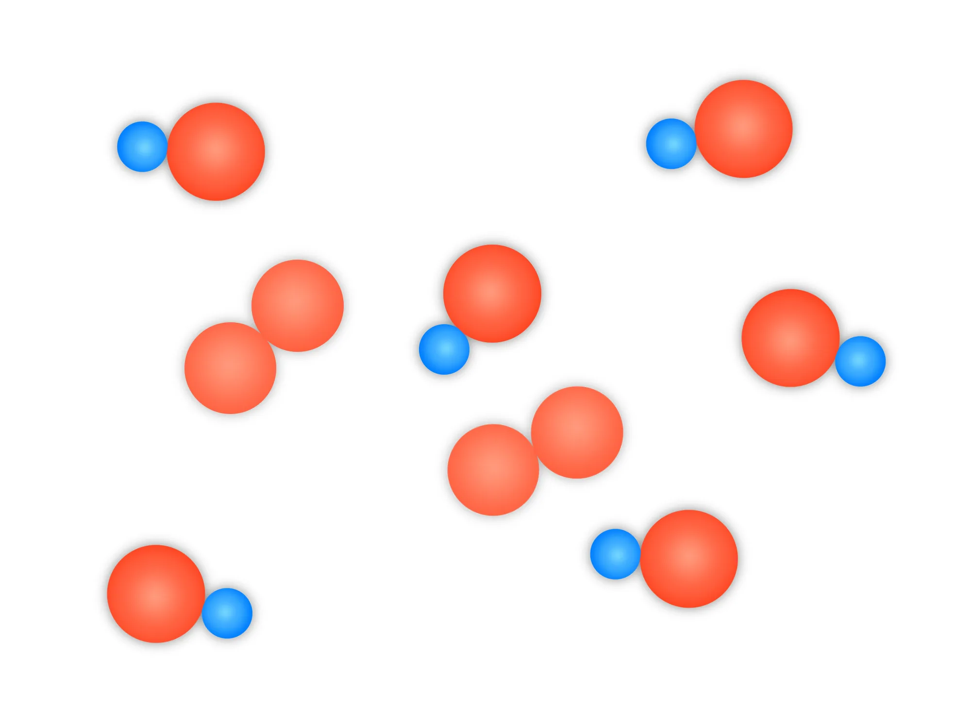
AP edition reviewed context. These retained source snapshots are unbalanced illustrations with unspecified species identities and sources or sinks: red pairs appear to increase from2 to5 while6 blue/red pairs remain unchanged. They do not establish a closed-system reaction or conservation of atoms. Do not infer a reaction time course or second-order law. Two drawn species do not establish rate-law powers; those require kinetic evidence or an explicitly established elementary step.
Read all reviewed image captions
Image 1
AP edition reviewed context. These retained source snapshots are unbalanced illustrations with unspecified species identities and sources or sinks: red pairs appear to increase from2 to5 while6 blue/red pairs remain unchanged. They do not establish a closed-system reaction or conservation of atoms. Do not infer a reaction time course or second-order law. Two drawn species do not establish rate-law powers; those require kinetic evidence or an explicitly established elementary step.
Image 2
AP edition reviewed context. These retained source snapshots are unbalanced illustrations with unspecified species identities and sources or sinks: red pairs appear to increase from2 to5 while6 blue/red pairs remain unchanged. They do not establish a closed-system reaction or conservation of atoms. Do not infer a reaction time course or second-order law. Two drawn species do not establish rate-law powers; those require kinetic evidence or an explicitly established elementary step.
Interactive 3.3.1 Second-Order
Read all reviewed figure notes
Non-Linear
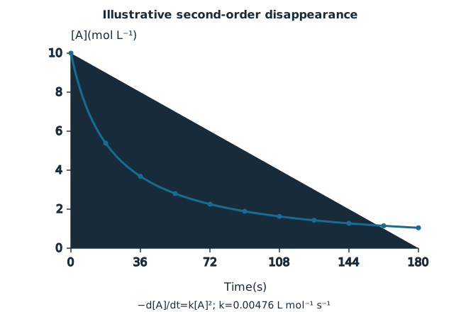
The specified −d[A]/dt=k[A]² model has a curved concentration plot. A straight reciprocal plot, rather than curve appearance alone, supports this law.
A second order rate constant, , has units of , and remains the same as it has always been:
−d[A]/dt=k[A]² is the disappearance law used here. The minus sign makes the disappearance rate positive when [A] decreases. A normalized reaction rate may differ by a stoichiometric factor.
For a Second-Order rate equation, if you were to graph , you would see a scatterplot that looks something like this:
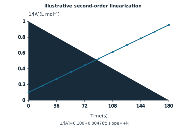
For −d[A]/dt=k[A]², plot 1/[A] in L mol⁻¹ versus t in s. It is linear with positive slope k in L mol⁻¹ s⁻¹. A general law k[A][B] does not automatically have this integrated form.
Interactive 3.3.2 Second-Order
Read all reviewed figure notes
Initial Measurement
The vertical axis is the reciprocal concentration1/[A], not a visually inverted concentration axis. Its units are L mol⁻¹. At t=0 it is1/[A]₀.
Positively Sloped
As reactant[A] decreases,1/[A] increases. For the specified law this gives a straight line with positive slope k in L mol⁻¹ s⁻¹.
Once again, we will investigate the cause of this relationship by integrating the rate equation to find the integrated second-order rate equation.
Let’s start with the second form of the rate equation and integrate that:
Now to solve for C, set time to 0, making :
Finally, plugging this in gives us the following:
This is our Integrated Second-Order Rate Equation.
The reciprocal law applies to −d[A]/dt=k[A]². It also applies to −d[A]/dt=k[A][B] if [A]=[B] throughout the interval.
For a fixed-volume 1:1 reaction A+B→products, equal initial concentrations remain equal if there are no other sources or sinks. Then k[A][B]=k[A]². Unequal initial concentrations or different stoichiometric consumption require a different integration.
Now it’s time to figure out the half-life equation for a second-order reaction. Starting with our integrated rate equation:
Set :
There is our formula for the half-life of a second-order reaction.
Reviewed replacement, Example3.3.1: A hypothetical fixed-volume NO₂ disappearance model specifies −d[NO₂]/dt=(12 L mol⁻¹ s⁻¹)[NO₂]² and [NO₂]₀=0.0030 M. Find the half-life. This explicitly defines k on the disappearance basis and does not claim a measured nitrogen/oxygen catalytic-converter mechanism.
As we are given , we can easily solve for :
t½=1/(k[NO₂]₀)=1/(12×0.0030)=27.7778 s≈28 s. If k instead defined the normalized reaction rate for2 NO₂, a factor of2 would enter disappearance; the reviewed prompt specifies its convention.
Reviewed replacement, Example3.3.2: In a hypothetical fixed-volume model for A+B→P, [A]₀=[B]₀=6.00 M and −d[A]/dt=k[A][B]. Successive intervals to halve the remaining concentration are35.0,70.0 and140.0 s. The cumulative times to [A]₀/2, [A]₀/4 and [A]₀/8 are35.0,105.0 and245.0 s. Determine k. These formal data replace the source’s inconsistent35,70,105 successive intervals and are not a precipitation procedure. The actual sodium carbonate formula is Na₂CO₃; calcium carbonate is CaCO₃.
| Transition | Interval(s) | Cumulative time(s) |
|---|---|---|
| 6.00→3.00 M | 35.0 | 35.0 |
| 3.00→1.50 M | 70.0 | 105.0 |
| 1.50→0.750 M | 140.0 | 245.0 |
For the declared model −d[A]/dt=k[A]², successive halving intervals double. Merely observing increasing intervals does not establish second order.
The first halving interval obeys t½=1/(k[A]₀).
Use the first interval35.0 s and initial concentration6.00 M.
Both concentrations are specified equal in the formal fixed-volume model; the1:1 consumption keeps them equal.
No salt mass or water-volume assumption is needed: [A]₀=6.00 M is explicitly supplied.
Use [A]₀=6.00 mol L⁻¹. This is formal model data, not a claim of realistic concentrated precipitation kinetics.
Solve for k using the first halving interval.
k=1/([A]₀t½).
k=1/(6.00×35.0).
k=0.00476190476 L mol⁻¹ s⁻¹≈0.00476 L mol⁻¹ s⁻¹. At3.00 M the interval is70.0 s; at1.50 M it is140.0 s. The original105 s third interval was inconsistent with this law.
If one reactant’s concentration stays effectively constant over the measured interval, absorb its concentration factor into an effective constant. This is a pseudo-order approximation; it does not change the underlying empirical law.
For an illustrative A+B→P reaction with measured disappearance law k[A][B], consider B in sufficient excess that its fractional change is negligible. This generic model is clearer than inferring methane combustion kinetics from its balanced equation.
The reviewed generic stoichiometry is A+B→P. It is separate from a real methane combustion mechanism; stoichiometry alone cannot establish that reaction’s rate law.
Excess means the concentration change is small enough for the desired accuracy; it does not mean exactly constant automatically. A controlled reservoir can also hold [B] fixed. Check that condition before using a pseudo-first-order law.
Suppose kinetic data establish −d[A]/dt=k[A][B]. We are declaring this law; coefficients alone do not establish it.
With [B]≈[B]fixed, −d[A]/dt=k′[A], where k′=k[B]fixed and k′ has inverse-time units. The model is pseudo-first order in A within that range.
Here’s a list of all the equation for the Zeroth-Order, First-Order, and Second-Order reactions:
Zeroth-Order:
The rate equation:
The integrated rate equation:
The half-life equation:
First-Order:
The rate equation:
The integrated rate equation:
The half-life equation:
Second-Order:
Second-order summary: for −d[A]/dt=k[A]², 1/[A]=1/[A]₀+kt and t½=1/(k[A]₀). The same form applies to k[A][B] only when [A]=[B] throughout. These formulas use the explicitly declared species-disappearance convention.
Glossary and deeper reading · 9 refreshers
These editorial refreshers supplement the reading. Definitions and examples are added guidance; original source wording and recorded answers remain in their original context.
-
Reaction order
Reaction order describes the concentration dependence in a rate law. An order in one reactant is its exponent, and overall order is the sum of the concentration exponents. For example, a second-order dependence on one reactant makes quadrupling the rate follow from doubling that reactant's concentration under fixed conditions.
-
Reaction half-life
A reaction half-life is the time needed for a reactant's concentration to fall to half its starting value under the specified model. A first-order reaction has a half-life independent of its starting concentration, while other orders generally do not. For example, consecutive equal time intervals halve a first-order reactant's concentration repeatedly.
-
Elementary reaction
An elementary reaction is one step in a proposed mechanism rather than the sum of multiple steps. For a specified elementary step, the rate-law concentration factors follow its reacting-particle event. For example, a bimolecular elementary collision can have a rate proportional to the concentrations of its two reactants.
-
Rate constant
A rate constant is the proportionality factor in a specified rate law. Its value depends on conditions such as temperature, and its units depend on the law's overall order. For example, a first-order rate constant has units of inverse time when concentration is measured per unit volume.
-
Reaction rate
Reaction rate describes how quickly a reactant or product quantity changes with time. Rates expressed using different species must account for their stoichiometric coefficients. For example, a product's concentration–time slope can be used to determine its rate of formation.
-
Stoichiometry
Stoichiometry uses a balanced chemical equation to relate amounts of reactants and products. Equation coefficients provide mole ratios rather than direct mass ratios. For example, forming water from hydrogen and oxygen consumes two moles of hydrogen molecules per mole of oxygen molecules.
-
Precipitate
A precipitate is a solid phase that forms from species in a solution. Whether it forms depends on the ion concentrations and the relevant equilibrium conditions. For example, silver ions and chloride ions can produce a silver chloride precipitate.
-
Mole
A mole is an amount of substance containing exactly 6.02214076 × 10²³ specified entities. The entities can be atoms, molecules, ions, or formula units, so the counted entity must be named. For example, one mole of oxygen molecules contains two moles of oxygen atoms.
-
Rate law
A rate law relates a reaction rate to reactant concentrations and a rate constant under stated conditions. For an overall reaction, its concentration exponents are established from evidence rather than copied from the balanced equation. For example, doubling one reactant concentration doubles the rate when the reaction is first order in that reactant and other conditions are fixed.